1 item has been added to your cart.
Populations are often divided into groups or subpopulations—age groups, income brackets, levels of education. Regression models or distributions likely differ across these groups. But sometimes we don't have a variable that identifies the groups. Perhaps the identifying variable is simply missing. Perhaps it is hard to collect—honest reporting of drug use, sex of goldfish, etc. Perhaps it is inherently unobservable—penchant for risky behavior, high propensity to save money, etc. In such cases, we can use finite mixture models (FMMs) to model the probability of belonging to each unobserved group, to estimate distinct parameters of a regression model or distribution in each group, to classify individuals into the groups, and to draw inferences about how each group behaves.
For instance, we might want to model an individual's annual number of doctor visits based on age and medical conditions. However, the model is likely to differ for individuals who are inclined to schedule an appointment at the first sign of a problem compared with those who wait until conditions are more serious. An automobile insurance company might want to classify drivers into risk categories. Those categories may be high and low risk, or they may be high, medium, and low risk. With FMMs, we can estimate the probability of belonging to a group and fit group-specific models.
Let's continue with the insurance company example. If we are interested in fitting a linear regression model, say,
. regress y x1 x2 x3
and believe that there are two risk categories, we could add the fmm: prefix,
. fmm 2: regress y x1 x2 x3
and fit a mixture of two regression models.
fmm: can be used with other estimators too. In the above example, y is a continuous outcome. If y were binary—it might stand for having an accident or not having one—we could type
. fmm 2: logit y x1 x2 x3
or
. fmm 2: probit y x1 x2 x3
If y were a count outcome, we could type
. fmm 2: poisson y x1 x2 x3
If we thought there were three risk categories, we could type
. fmm 3: poisson y x1 x2 x3
We have fictional data on automobile insurance claims. Our data record the number of accidents drivers had in a year:
. tabulate accident
| accident | Freq. Percent Cum. | |
| 0 | 2,079 42.35 42.35 | |
| 1 | 1,402 28.56 70.91 | |
| 2 | 689 14.04 84.95 | |
| 3 | 357 7.27 92.22 | |
| 4 | 152 3.10 95.31 | |
| 5 | 121 2.46 97.78 | |
| 6 | 72 1.47 99.25 | |
| 7 | 37 0.75 100.00 | |
| Total | 4,909 100.00 |
We want to model the number of accidents based on age, sex, and whether the individual lives in a metropolitan area. We are thinking about fitting the model
. poisson accident c.age##c.age i.metro i.male
We hypothesize, however, that there are two groups of drivers: risky ones and cautious ones. If we are right, the Poisson model would differ across the two groups. We cannot include the driver risk group because risk group is inherently unobservable.
So instead, we fit a finite mixture of two Poisson regressions:
. fmm 2: poisson accident c.age##c.age i.metro i.male

Finite mixture model                            Number of obs     =      4,909
Log likelihood = -6830.4939
| Coef. Std. Err. z P>|z| [95% Conf. Interval] | ||||
| 1.Class | (base outcome) | |||
| 2.Class | (base outcome) | |||
| _cons | 1.292315 .1456052 8.88 0.000 1.006934 1.577696 | |||
| Coef. Std. Err. z P>|z| [95% Conf. Interval] | ||||
| accident | ||||
| age | .945157 .6395391 1.48 0.139 -.3083167 2.198631 | |||
| c.age#c.age | -.3188467 .1289995 -2.47 0.013 -.5716811 -.0660123 | |||
| 1.metro | .2705157 .0541961 4.99 0.000 .1642932 .3767381 | |||
| 1.male | .6090904 .0557893 10.92 0.000 .4997455 .7184353 | |||
| _cons | .113725 .7817361 0.15 0.884 -1.41845 1.6459 | |||
| Coef. Std. Err. z P>|z| [95% Conf. Interval] | ||
| accident | ||
| age | -.7687128 .5466519 -1.41 0.160 -1.840131 .3027052 | |
| c.age#c.age | -.0393748 .1119022 -0.35 0.725 -.2586992 .1799495 | |
| 1.metro | .741119 .0484484 15.30 0.000 .6461619 .836076 | |
| 1.male | .6094243 .0495992 12.29 0.000 .5122117 .7066369 | |
| _cons | 1.140167 .6553976 1.74 0.082 -.144389 2.424722 | |
There are three parts to the output: (1) results of a model for the unobserved group variable, (2) the Poisson model for accidents in the first group, and (3) the Poisson model for accidents in the second group.
The technical jargon for the two unobserved groups is latent class. That is why the first part of the output shows results for Class, 1.Class, and 2.Class. Class is the unobserved variable. 1.Class is its first group, and 2.Class is its second group just as it would be had Class been a real Stata variable.
In parts two and three of the output, the fitted Poisson models are reported. You interpret the coefficients in them just as you would if you had fit two separate Poisson models.
So which class represents risky drivers? Do the two classes have anything even to do with riskiness? We can use estat lcmean to estimate the expected number of accidents in each class:
. estat lcmean

Latent class marginal means                     Number of obs     =      4,909
| Delta-method | ||||
| Margin Std. Err. z P>|z| [95% Conf. Interval] | ||||
| 1 | ||||
| accident | 2.605624 .1275088 20.43 0.000 2.355712 2.855537 | |||
| 2 | ||||
| accident | .7749165 .0290796 26.65 0.000 .7179215 .8319114 | |||
Members of class 1 are expected to have 2.6 accidents per year.
Members of class 2 are expected to have 0.8 accidents per year.
Class membership certainly has to do with expected accident rate, and we take that as evidence that the classes provide some indication of riskiness.
Let's continue with that interpretation and ask what proportion of drivers are risky.
. estat lcprob

Latent class marginal probabilities                     Number of obs     =      4,909
| Delta-method | ||||
| Margin Std. Err. [95% Conf. Interval] | ||||
| Class | ||||
| 1 | .2154612 .0246128 .171122 .2675803 | |||
| 2 | .7845388 .0246128 .7324197 .828878 | |||
The answer is that 22% are risky.
We can visually compare the distributions of predicted insurance claims for the two classes:
. predict mu*
(option mu assumed)

. twoway histogram mu1, width(.25) color(navy%25)
         histogram mu2, width(.25) color(maroon%25)
         legend(off) title("Predicted number of claims for two groups")
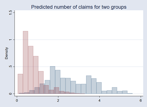
We can see that the two groups differ.
In the example, we did not assume much about driver riskiness except that it would cause different Poisson models to be fit. The story about the riskiness of drivers is perhaps appealing, but all we did was ask about heterogeneity in our data and discovered that there was enough that, if the data were divided in the right way, the Poisson models would differ.
We can also specify variables on which class membership is to be modeled. We fit the model in the example by typing
. fmm 2: poisson accident c.age##c.age i.metro i.male
Had we typed
        . fmm 2, lcprob(i.age16to18 i.skydives i.smokes):
                 poisson accident c.age##c.age i.metro i.male
class membership would also be determined by the specified variables in a multinomial logit model.
When you type
. fmm 2: poisson accident c.age##c.age i.metro i.male
you are fitting the model for two groups. The models for the groups do not have to contain the same variables. You could type
. fmm: ( poisson accident c.age##c.age i.metro i.male )
       ( poisson accident c.age##c.age         i.male )
This is no different from placing constraints on individual equations.
The two models do not have to use the same estimation command. You could use different commands with different distributional assumptions. You could type
. fmm: ( poisson accident c.age##c.age i.metro i.male )
       ( nbreg   accident c.age##c.age         i.male )
All this can be combined with option lcprob() to specify the class model:
. fmm,    lcprob(i.age16to18 i.skydives i.smokes):
          ( poisson accident c.age##c.age i.metro i.male )
          ( nbreg   accident c.age##c.age         i.male )
Learn more about Stata's finite mixture models features.
Read more about finite mixture models in the Stata Finite Mixture Models Reference Manual; see [FMM] fmm intro.