Generalized linear responses
Continuous—linear, gamma
Binary—probit, logit, complementary log-log
Count—Poisson, negative binomial, truncated Poisson
Categorical—multinomial logit
Ordered—ordered logit, ordered probit
Censored continuous
Fractional—beta
Survival-time—exponential, loglogistic, Weibull, lognormal, gamma
Multilevel data
Nested: two levels, three levels, more levels
Hierarchical
Crossed
Latent variables at different levels
Random intercepts
Random slopes
Mixed models
Multiple-group models
Easily specify groups
Constrain groups of parameters to be equal across groups
Test for group invariance
Meaning you can fit
CFA with binary, count, and ordinal measurements
Multilevel CFA
Multilevel mediation
Item response theory (IRT)
Latent growth curves with repeated measurements of binary, count, and ordinal responses
Selection models
Endogenous treatment effects
Multilevel survival models
Survival models with latent predictors
Any multilevel SEM with generalized linear responses
Support for survey data
Sampling weights
Clustering
Stratification
Finite-population corrections
Stata's sem command fits linear SEM.
Stata's gsem command fits generalized SEM, by which we mean (1) SEM with generalized linear response variables and (2) SEM with multilevel mixed effects, whether linear or generalized linear.
Generalized linear response variables mean you can fit logistic, probit, Poisson, multinomial logistic, ordered logit, ordered probit, beta, and other models. It also means measurements can be continuous, binary, count, categorical, ordered, fractional, and survival times.
Multilevel mixed effects means you can place latent variables at different levels of the data. You can fit models with fixed or random intercepts and fixed or random slopes.
Say we have a test designed to assess mathematical performance. The data record a set of binary variables measuring whether individual answers were correct. The test was administered to students at various schools.
We postulate that performance on the questions is determined by unobserved (latent) mathematical aptitude and by school quality, representing unmeasured characteristics of the school:
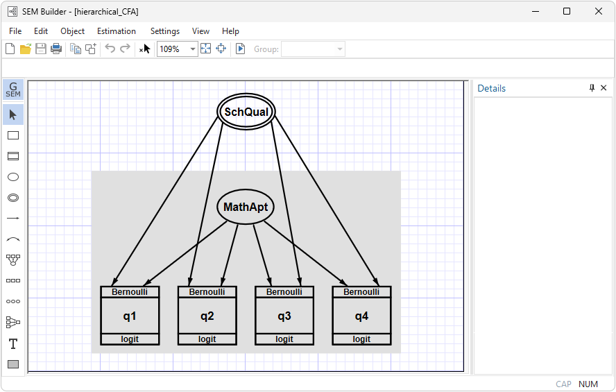
In the diagram, the values of the latent variable SchQual are constant within school and vary across schools.
We can fit the model from the path diagram by pressing  . Results will appear on the diagram.
Or, we can skip the diagram and type the equivalent command
. gsem (MathApt -> q1 q2 q3 q4) (SchQual[school] -> q1 q2 q3 q4), logit
Either way, we get the same results:
Generalized structural equation model                          Number of obs = 500

(output omitted)

Log likelihood = -1348.3644

 ( 1)  [q1]SchQual[school] = 1
 ( 2)  [q2]MathApt = 1
| Coefficient Std. err. z P>|z| [95% conf. interval] | ||
| q1 | ||
| SchQual[school] | 1 (constrained) | |
| MathApt | 5.277956 4.995708 1.06 0.291 -4.513451 15.06936 | |
| _cons | .0413352 .1770215 0.23 0.815 -.3056206 .3882909 | |
| q2 | ||
| SchQual[school] | .600067 .3447607 1.74 0.082 -.0756516 1.275786 | |
| MathApt | 1 (constrained) | |
| _cons | -.449189 .1165887 -3.85 0.000 -.6776987 -.2206793 | |
| q3 | ||
| SchQual[school] | .3999959 .3008142 1.33 0.184 -.1895891 .989581 | |
| MathApt | 1.788696 1.10452 1.62 0.105 -.3761236 3.953516 | |
| _cons | .1485335 .1070996 1.39 0.165 -.0613779 .3584449 | |
| q4 | ||
| SchQual[school] | .5925695 .34909 1.70 0.090 -.0916343 1.276773 | |
| MathApt | 1.071626 .7310121 1.47 0.143 -.3611311 2.504384 | |
| _cons | -.3203425 .1152657 -2.78 0.005 -.5462592 -.0944258 | |
| var(Sch~l[sch~l]) | .2483231 .24206 .0367523 1.677838 | |
| var(MathApt) | .1050076 .1133871 .0126501 .8716606 | |
Math aptitude has a larger variance and loadings than school quality. Thus math aptitude is more important than school, although school is still important.
See Structural Equation Modeling Reference Manual and especially see the introduction.
Watch the videos:
Tour of multilevel generalized SEM in StataDon't miss the 28 worked examples demonstrating generalized SEM:
Single-factor measurement model (generalized response)
One-parameter logistic IRT (Rasch) model
Two-parameter logistic IRT model
Two-level measurement model (multilevel, generalized response)
Two-factor measurement model (generalized response)
Full structural equation model (generalized response)
Logistic regression
Combined models (generalized responses)
Ordered probit and ordered logit
MIMIC model (generalized response)
Multinomial logistic regression
Random-intercept and random-slope models (multilevel)
Three-level model (multilevel, generalized response)
Crossed models (multilevel)
Two-level multinomial logistic regression (multilevel)
One- and two-level mediation models (multilevel)
Tobit regression
Interval regression
Heckman selection model
Endogenous treatment-effects model
Exponential survival model
Loglogistic survival model with censored and truncated data
Multiple-group Weibull survival model
Latent class model
Latent class goodness-of-fit statistics
Latent profile model
Finite mixture Poisson regression
Finite mixture Poisson regression, multiple responses


