The new bayes: qreg command fits Bayesian quantile regression, which allows you to incorporate prior information about the quantile coefficients.

Quantile regression models the conditional quantiles of an outcome as a linear combination of predictors. Traditional quantile regression relies on a specific set of loss functions and linear programming for estimation. To introduce Bayesian quantile regression, Yu and Moyeed (2001) use an equivalent formulation of the quantile regression loss function that assumes an asymmetric Laplace distribution for the likelihood function of the data. Bayesian quantile regression combines this likelihood formulation with priors for model parameters to form a posterior model and uses Markov chain Monte Carlo (MCMC) for estimation. This provides full posterior distributions of model parameters for comprehensive inference.

In classical quantile regression, standard errors are computed by using bootstrap or kernel-based methods. In the Bayesian framework, posterior standard deviations play the role of standard errors. By assuming a parametric likelihood model, the posterior standard deviations are estimated based on that model and may be more efficient under the correct likelihood specification.

In practice, the assumption of an asymmetric Laplace distribution for the conditional distribution of the outcome given the covariates is often too restrictive in the context of quantile regression and may lead to model misspecification (Yang, Wang, and He 2016; Ji, Lee, and Rabe-Hesketh 2025). The posterior mean and mode estimates are still valid under model misspecification (Sriram, Ramamoorthi, and Ghosh 2013), but the posterior standard deviations are too small and credible intervals are too narrow. To address underestimation of the variability, Yang, Wang, and He (2016) proposed an adjustment to the variance–covariance matrix of the quantile coefficients from the asymmetric Laplace model. The adjustment can be viewed as an asymptotically normal approximation of the true posterior distribution. Thus, the inference should be based on the so-called adjusted variance–covariance matrix and adjusted credible intervals when the assumption of the asymmetric Laplace model is suspect. In what follows, we refer to the results based on the approximating normal model as adjusted quantile coefficients, adjusted standard errors, and adjusted credible intervals.

Let's see it work

Let's explore the relationship between household income and food expenditure using the data from Engel (1857), which are described in Koenker and Bassett (1982). Let's use a quantile regression to compare this relationship across different quantiles. We first fit a model to the 50th percentile of the outcome variable, a model known as median regression, using default settings. We specify the rseed(19) option for reproducibility.

. webuse engel1857
(European household budget survey)

. bayes, rseed(19): qreg foodexp income

Burn-in ...
Simulation ...

Model summary


Likelihood:
foodexp ~ asymlaplaceq(xb_foodexp_q50_al,{sigma_al},.5)

Priors:
  {foodexp_q5~l:income _cons} ~ normal(0,10000)                              (1)
                   {sigma_al} ~ igamma(0.01,0.01)

(1) Parameters are elements of the linear form xb_foodexp_q50_al.
Bayesian quantile regression                       MCMC iterations  =     12,500
Metropolis–Hastings and Gibbs sampling             Burn-in          =      2,500
                                                   MCMC sample size =     10,000
Quantile = .5                                      Number of obs    =        235
                                                   Acceptance rate  =      .5735
                                                   Efficiency:  min =     .09896
                                                                avg =       .151
Log marginal-likelihood =  186.43947                            max =      .2268



               
 
                                                Equal-tailed    
               
 
      Mean   Std. dev.     MCSE     Median  [95% cred. interval]
 
 
 
foodexp_q50_al 
 
                                                                
        income 
 
  .5567276   .0159401   .000507   .5562547   .5248025    .587735
         _cons 
 
   .084986   .0143782   .000403   .0851108   .0575581   .1134264
 
 
 
      sigma_al 
 
  .0377533   .0024907   .000052   .0376511   .0331066   .0430957

Warning: Posterior model uses asymmetric Laplace likelihood, which may be
         misspecified for quantile regression.

Posterior summaries using normal approximation



             
 
                                                Equal-tailed    
 foodexp_q50 
 
      Mean   Std. dev.     MCSE     Median  [95% cred. interval]
 
 
 
      income 
 
  .5568266    .027778   .000274   .5567865   .5037128   .6111692
       _cons 
 
  .0849174   .0224273    .00022   .0848101   .0413198   .1285213

The command reports two output tables. The parameters in the first table, {foodexp_q50_al:} and {sigma_al}, correspond to the quantile coefficients and scaling factor, respectively, based on the asymmetric Laplace likelihood. The parameters in the second table, {foodexp_q50:}, are the adjusted quantile coefficients, which we use for inference.

The mean posterior estimate for the coefficient of income is 0.56 with a 95% credible interval (CrI) of [0.50, 0.61]. We now shift our attention to the 25th percentile (or 0.25 quantile) of the outcome variable by specifying the quantile() option with qreg.

. bayes, rseed(19): qreg foodexp income, quantile(0.25)

Burn-in ...
Simulation ...

Model summary


Likelihood: 
Likelihood:
  foodexp ~ asymlaplaceq(xb_foodexp_q25_al,{sigma_al},.25)

Priors:
  {foodexp_q2~l:income _cons} ~ normal(0,10000)                              (1)
                   {sigma_al} ~ igamma(0.01,0.01)

(1) Parameters are elements of the linear form xb_foodexp_q25_al.

Bayesian quantile regression                       MCMC iterations  =     12,500
Metropolis–Hastings and Gibbs sampling             Burn-in          =      2,500
                                                   MCMC sample size =     10,000
Quantile = .25                                     Number of obs    =        235
                                                   Acceptance rate  =      .5615
                                                   Efficiency:  min =      .1436
                                                                avg =      .1765
Log marginal-likelihood =  169.18624                            max =      .2421



               
 
                                                Equal-tailed    
               
 
      Mean   Std. dev.     MCSE     Median  [95% cred. interval]
 
 
 
foodexp_q25_al 
 
                                                                
        income 
 
  .4718604   .0140225    .00037   .4735463   .4414884   .4948657
         _cons 
 
  .0962851   .0116976   .000308   .0957929   .0742573   .1196877
 
 
 
      sigma_al 
 
  .0304463   .0020364   .000041   .0303373   .0266857   .0347907

Warning: Posterior model uses asymmetric Laplace likelihood, which may be
         misspecified for quantile regression.

Posterior summaries using normal approximation



             
 
                                                Equal-tailed    
 foodexp_q25 
 
      Mean   Std. dev.     MCSE     Median  [95% cred. interval]
 
                                                                
      income 
 
  .4719483   .0246847   .000243   .4719127   .4247493   .5202395
       _cons 
 
  .0962404   .0163897   .000164    .096187   .0644156    .128502

The mean posterior estimate for the coefficient of income is 0.47 with a 95% CrI of [0.42, 0.52].

We also fit a quantile regression for the 75th percentile (or 0.75 quantile).

. bayes, rseed(19): qreg foodexp income, quantile(0.75)

Burn-in ...
Simulation ...

Model summary


Likelihood: 
  foodexp ~ asymlaplaceq(xb_foodexp_q75_al,{sigma_al},.75)

Priors: 
  {foodexp_q7~l:income _cons} ~ normal(0,10000)                             (1)
                   {sigma_al} ~ igamma(0.01,0.01)

(1) Parameters are elements of the linear form xb_foodexp_q75_al.

Bayesian quantile regression                      MCMC iterations  =     12,500
Metropolis–Hastings and Gibbs sampling            Burn-in          =      2,500
                                                  MCMC sample size =     10,000
Quantile = .75                                    Number of obs    =        235
                                                  Acceptance rate  =      .5402
                                                  Efficiency:  min =      .1421
                                                               avg =      .1704
Log marginal-likelihood =  188.25668                           max =      .2262



              
 
                                                Equal-tailed    
              
 
      Mean   Std. dev.     MCSE     Median  [95% cred. interval]
 
 
 
foodexp_q75~l 
 
                                                                
       income 
 
  .6456717   .0170002   .000451   .6461026   .6089782   .6757706
        _cons 
 
  .0606789    .014418   .000381    .060412    .034519   .0924086
 
 
 
     sigma_al 
 
  .0280768   .0018942    .00004   .0279643   .0245888   .0321131

Warning: Posterior model uses asymmetric Laplace likelihood, which may be
         misspecified for quantile regression.

Posterior summaries using normal approximation



             
 
                                                Equal-tailed    
 foodexp_q75 
 
      Mean   Std. dev.     MCSE     Median  [95% cred. interval]
 
 
 
      income 
 
  .6458052   .0374615   .000369   .6457512   .5741757    .719092
       _cons 
 
  .0605835   .0290556   .000287   .0604811   .0039029   .1163959

The mean posterior estimate for the coefficient of income is 0.65 with a 95% CrI of [0.57, 0.72]. If we compare the CrIs for the income coefficients from the last two quantile regressions, they are not overlapping, which suggests that the relationship between income and food expenditure is different between the 0.25 and 0.75 quantiles.

We can explore this relationship further by specifying different quantiles in the quantile() option with bayes: qreg and using the results to produce the graph below:

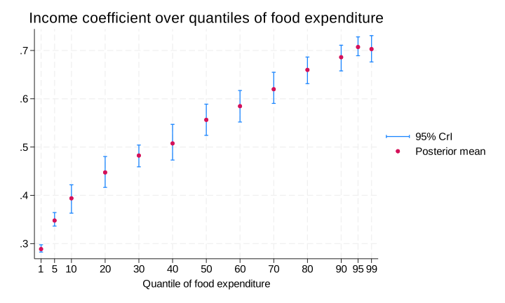
The graph demonstrates heterogeneity of the income coefficients across the distribution (quantiles) of food expenditure. The coefficient increases as the quantile value increases. (This does not mean that the proportion of income spent on food increases with income. If we were to obtain predictions and produce the Engel curve, we would see that food expenditure share decreases with income, as expected.)

All existing Bayesian postestimation commands are available after bayes: qreg, except bayespredict and bayesstats ppvalues. For example, we can compute the posterior probability for the income coefficient in the model for the 25th percentile of foodexp to be within the interval [0.574, 0.719]—the 95% CrI obtained from the 75th percentile regression model. To accomplish this, we use the bayestest interval command.

. bayestest interval {foodexp_q25:income}, lower(.574) upper(.719)

Interval tests     MCMC sample size =    10,000

       prob1 : .574 < {foodexp_q25:income} <
               .719



             
 
      Mean    Std. dev.      MCSE
 
 
 
       prob1 
 
         0     0.00000          0

The estimated posterior probability is 0, which suggests that the effect of income on food expenditure differs between the 25th and 75th percentiles.