If you have a multivalued treatment or groups that switch in and out of treatment, traditional difference-in-differences (DID) estimators are of little use. The new xtswitchdid command handles both multivalued and switching treatments and allows you to explore treatment paths across groups over time. As with other DID estimators, you can test parallel trends, plot results, aggregate effects, and more. This feature is a part of StataNow™.

Researchers often want to study the effects of a treatment, such as a policy or intervention, on a group, exploiting variation in the timing or presence of treatment. In many applications, the treatments that are of interest are multivalued. They may be switching (nonabsorbing), meaning that after entering treatment, a treated group may transition to a higher or lower level of treatment or exit treatment altogether.

The xtswitchdid command allows for DID estimation of event-study treatment effects, even when treatments are multivalued or switching. These event-study effects are a measure of how the outcome changes when a group has been exposed to a treatment switch after a given number of periods, relative to a counterfactual in which a group experienced no treatment switch. In contrast, Stata's panel DID commands xtdidregress and xthdidregress estimate average treatment effects on the treated (ATET) for binary and absorbing treatments.

Let's see it work

We have fictional data on hockey teams in 30 minor hockey leagues in North America and are interested in the effect of the number of new safety protocols (safety) implemented at the league level on the number of player injury days per team each season (injrate), normalized by season length. We hypothesize that exposure to these safety protocols reduces injrate. Each safety protocol is a rule change made at the league level. For example, a rule requiring mouthguards or a rule setting a minimum age for body checking.

Our panel has 462 teams across the 30 leagues, each of which is observed for some of or all the years between 2010 and 2025 except for 2020, a pandemic year where outcomes and covariates are missing for all teams. We also observe the region in which each league is located (region), the team win percentages each season transformed by the logit function (lwinpct), and a measure of the intensity of each team’s schedule (schedule).

We xtset our data to identify the panel and time variables and fit a model for the effect of safety on injrate, using lwinpct and schedule as covariates.

. webuse hockey
(Fictional minor hockey team injury data)

. xtset team year

Panel variable: team (unbalanced)
 Time variable: year, 2010 to 2025
         Delta: 1 unit

. xtswitchdid (injrate lwinpct schedule) (safety), group(team)

Treatment and time information

Panel variable:  team
Time variable:   year
Time interval:   2010 thru 2025

Treatment level: team
Control:         safety maintaining baseline
Treatment:       safety changing from baseline



Initial      
 
                                                            
treatment    
 
      Groups          Obs   Switch out    Switch in    Absorbing
 
 
 
           0 
 
         272        3,749                     1 2 3           No
           1 
 
         140        1,956                       2 3           No
           2 
 
          50          723                         3          Yes



DID with switching treatments                         Number of obs    = 6,428
                                                      Number of panels =   462
                                                      Number of groups =   462

                                 (Std. err. adjusted for 462 clusters in team)


             
 
 Normalized    Robust                                           
             
 
     effect   std. err.      z    P>|z|     [95% conf. interval]
 
 
 
    Exposure 
 
                                                                
          1  
 
  -6.871766   2.679854    -2.56   0.010    -12.12418   -1.619348
          2  
 
   -2.75066   1.380428    -1.99   0.046     -5.45625   -.0450695
          3  
 
  -3.061524   .8162018    -3.75   0.000     -4.66125   -1.461798
          4  
 
  -1.038777   .7065305    -1.47   0.141    -2.423551    .3459975
          5  
 
  -.9033563   .5854862    -1.54   0.123    -2.050888    .2441756
          6  
 
  -1.140814   .4573033    -2.49   0.013    -2.037112   -.2445157
          7  
 
  -.9005077   .4021147    -2.24   0.025    -1.688638   -.1123773
          8  
 
  -1.239846   .4123365    -3.01   0.003    -2.048011   -.4316814
          9  
 
   .7121286   .9774432     0.73   0.466    -1.203625    2.627882
         10  
 
  -1.615785   .3346074    -4.83   0.000    -2.271603   -.9599661
         11  
 
  -1.405509    .457877    -3.07   0.002    -2.302931   -.5080862
         12  
 
  -1.613272    .430911    -3.74   0.000    -2.457842   -.7687025
         13  
 
  -1.213585   .3641668    -3.33   0.001    -1.927339   -.4998312
         14  
 
  -.3144064   .3203691    -0.98   0.326    -.9423183    .3135055

Note: Effects computed using covariates.

We specified this model using syntax similar to that of xthdidregress, where the outcome model is specified in the first set of parentheses and the treatment variable is specified in the second set. We use our panel variable team as our group variable here, but we could use a coarser group variable if we liked.

The header gives information about the model and the treatment variable. The initial treatment table shows that there are three values of the treatment variable for which we observe teams with that value as their initial treatment. This is important because our estimator computes differences only between groups that share an initial treatment value.

In this dataset, all treatment switches away from the initial treatment values are switches “into” treatment, meaning to a higher level of treatment rather than to a lower level. The “Switch in” column lists the values of treatment distinct from the initial treatment value that are eventually taken by teams with that initial treatment value. The “Absorbing” column indicates whether all teams with a particular initial treatment value have a treatment path that is absorbing, meaning teams that are treated remain treated in subsequent periods. In this case, this is true for teams with an initial treatment value of 2.

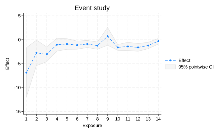
The table of results reports the normalized event-study effects of de Chaisemartin and D'Haultfœuille (2024). The effect at exposure 1 is the average effect on injrate of increasing safety by 1, as measured in the first treated period, relative to a counterfactual where the treatment had remained at the initial number of safety protocols.

Similarly, the effect at exposure 5 periods is the average effect of additional safety rules five periods after the most recent preswitch period, relative to a counterfactual where the treatment never changed from the initial value.

We can plot these effects using the postestimation command estat eventplot:

. estat eventplot

We may want to examine the treatment paths in the data and produce path-specific estimates for those that may be of interest. We can use the postestimation command estat paths to tabulate treatment paths:

. estat paths
note: pathlen() not specified; using path length 14.
note: variable _did_paths, which encodes a unique value for each treatment
      path, was added to the dataset.

Distribution of treatment paths

Path length: 14, not counting initial treatment
Treatment:   team changing initial treatment level


                        Paths 
 
      Freq.     Percent        Cum.
 
 
 
0 1 1 2 2 2 2 2 2 . 2 2 2 2 2 
 
         14        4.56        4.56
0 2 . 2 2 2 2 2 2 . . . . . . 
 
          1        0.33        4.89
0 2 2 2 . 2 2 2 2 . 2 3 3 3 3 
 
          3        0.98        5.86
0 2 2 2 2 2 0 0 . . 0 0 0 0 0 
 
          1        0.33        6.19
0 2 2 2 2 2 0 0 0 . 0 0 0 0 0 
 
         55       17.92       24.10
0 2 2 2 2 2 2 2 . . 2 3 3 3 3 
 
          1        0.33       24.43
0 2 2 2 2 2 2 2 . 2 3 3 3 3 . 
 
          1        0.33       24.76
0 2 2 2 2 2 2 2 2 . . . . . . 
 
         11        3.58       28.34
0 2 2 2 2 2 2 2 2 . . 3 3 3 3 
 
          2        0.65       28.99
0 2 2 2 2 2 2 2 2 . 2 3 3 3 . 
 
          1        0.33       29.32
0 2 2 2 2 2 2 2 2 . 2 3 3 3 3 
 
         82       26.71       56.03
0 3 3 3 3 . . . . . . . . . . 
 
         18        5.86       61.89
1 2 . 2 2 2 2 2 2 . 2 2 2 2 2 
 
          1        0.33       62.21
1 2 2 2 2 2 2 . 2 . 2 2 2 2 2 
 
          1        0.33       62.54
1 2 2 2 2 2 2 2 2 . . . . . . 
 
         16        5.21       67.75
1 2 2 2 2 2 2 2 2 . 2 . 3 3 3 
 
          1        0.33       68.08
1 2 2 2 2 2 2 2 2 . 2 2 2 2 2 
 
         30        9.77       77.85
1 2 2 2 2 2 2 2 2 . 2 3 3 3 3 
 
         57       18.57       96.42
2 3 3 3 . 3 3 3 3 3 . . . . . 
 
         11        3.58      100.00
 
 
 
                        Total 
 
        307      100.00            

The output shows us the treatment paths, starting from the last period before the treatment changed. We saw earlier that there was at least one treatment path that was not absorbing, and now we can see them in the output. The fourth- and fifth-listed paths show that there are 56 teams who switch into treatment (2 safety rules) and then switch back out of it after 5 periods.

If we run estat paths with the generate() option, it will produce an indicator variable for each path, which can be used in the path() option of xtswitchdid to produce path-specific estimates. See [CAUSAL] xtswitchdid for more details about this example. Below is the output when we request path-specific estimates for the fifth path in the table above:

. quietly estat paths, generate(safetypath)

. xtswitchdid (injrate lwinpct schedule) (safety), group(team) path(safetypath5)
(output omitted)

DID with switching treatments                         Number of obs    = 2,222
                                                      Number of panels =   268
                                                      Number of groups =   268
Treatment path: (0 2 2 2 2 2 0 0 0 . 0 0 0 0 0)
Treatment type: Switcher-in, nonabsorbing

                                 (Std. err. adjusted for 268 clusters in team)


             
 
 Normalized    Robust                                           
             
 
     effect   std. err.      z    P>|z|     [95% conf. interval]
 
 
 
    Exposure 
 
                                                                
          1  
 
  -8.803413   3.036455    -2.90   0.004    -14.75476    -2.85207
          2  
 
  -3.423294   1.351155    -2.53   0.011    -6.071509   -.7750789
          3  
 
  -2.574106   .9883007    -2.60   0.009     -4.51114   -.6370724
          4  
 
  -1.090292   .8124545    -1.34   0.180    -2.682673      .50209
          5  
 
  -.3275366   .6412151    -0.51   0.609    -1.584295    .9292218
          6  
 
  -1.138047   .5870595    -1.94   0.053    -2.288663    .0125683
          7  
 
   -1.17035   .5815419    -2.01   0.044    -2.310152   -.0305493
          8  
 
  -1.320975   .5834758    -2.26   0.024    -2.464567   -.1773839
          9  
 
          0  (omitted)                                          
         10  
 
  -.9877028   .5803887    -1.70   0.089    -2.125244    .1498381
         11  
 
  -.9415612    .927531    -1.02   0.310    -2.759489    .8763662
         12  
 
  -1.390374   .9659295    -1.44   0.150    -3.283561    .5028133
         13  
 
  -.3080592   .9232056    -0.33   0.739    -2.117509    1.501391
         14  
 
  -.8733448   .8459017    -1.03   0.302    -2.531282    .7845921

Note: effects computed using covariates.

The output now omits the first table about initial treatment groups because we are looking only at one path. The header displays the path, informing us that groups with this treatment path are switchers-in and that the treatment is nonabsorbing.