
← See Stata 19's new features
Highlights
Fit heterogeneous DID models for fractional, binary, and count outcomes
Model heterogeneity over cohort and time
Plot treatment-effects heterogeneity
Plot event-study estimates
Test of parallel pretreatment trends
Aggregate ATETs over
cohort,
time, and
exposure to treatment
Obtain moderating effects for covariates
See more causal inference features
Heterogeneous difference-in-differences (DID) modeling now goes beyond linear models. The new xthdidfracreg, xthdidlogit, and xthdidpoisson commands allow you to fit heterogeneous DID panel-data models for fractional, binary, and count outcomes by using estimators for nonlinear models. As with other DID commands, you can test for parallel pretreatment trends, aggregate heterogeneous ATETs within cohort and time, explore effects of exposure to treatment over time, and obtain moderating effects. These features are a part of StataNow™.
DID is an essential tool for researchers. It determines if an intervention at a point in time had a causal effect for those that were subject to an intervention and looks at these effects over time. DID is also appealing because you can validate identification with graphical diagnostics and tests.
In Stata, you can fit models for homogeneous DID, heterogeneous DID under staggered designs, and heterogeneous DID with switchers. Now we can also fit nonlinear heterogeneous DID models for binary, count, and fractional outcomes.
Suppose that we have panel data for a set of individuals across 10 years and we would like to study the effect of a change in policy. Different groups of individuals experienced the policy change at different times. We can use heterogeneous DID methods to estimate the ATET for each cohort at each point in time.
First, we use xtset to tell Stata that we have a panel dataset with individual identifiers stored in the idcode variable and time stored in the year variable.
. xtset idcode year
Now we can obtain the ATET estimates for a binary outcome ybin by using the xthdidlogit command.
. xthdidlogit (ybin x1) (policy), group(county)
Or if we have a count outcome ycount, we could type
. xthdidpoisson (ycount x1) (policy), group(county)
Or if we have a fractional outcome yfrac, we could type
. xthdidfracreg logit (yfrac x1) (policy), group(county)
These commands automatically identify the cohorts—the individuals that were treated at the same time. However, you may instead create and specify a variable that identifies the cohorts. To create a cohort variable named mycohort before estimation, we type
. gencohort mycohort, group(county) time(year) treat(policy)
and then add the usercohort(mycohort) option to our xthdidlogit, xthdidpoisson, or xthdidfracreg command. This is beneficial if you have missing data or other challenges in your data that could affect the automated identification of cohorts or if you want to analyze cohorts before fitting the model.
After estimation with any of the three commands, we can test assumptions and further interpret the results.
We can visualize the estimated ATETs by typing
. estat atetplot
We may want to aggregate the treatment effects over time or over cohort or even over time and cohort to obtain an overall ATET. We would type
. estat aggregation, cohort
or
. estat aggregation, time
or
. estat aggregation, overall
We can test for parallel pretreatment trends by typing
. estat ptrends
And we can estimate moderating effects that tell us how the ATET changes with covariates by typing
. estat moderation
First, we consider using a logit model to estimate ATETs for a binary outcome. We are interested in modeling the effect of having no social media apps (nosmapps) on high levels of stress (hstress) for a panel of high-school students. hstress is based on a diagnostic test and is 0 if the student does not experience a high level of stress and 1 otherwise. The school district promoted eliminating social media apps from phones starting in 2014. Throughout the time of the study, some students opted to follow the suggestion while others did not. For controls, we incorporate the hours exercised each week (exercise) and if the student participates in a group activity (gactivity). Group activities could be sports, after-school activities, or clubs, none of which are necessarily sponsored by the school.
First, we tell Stata that we have a panel dataset of individuals (id) over year. We type
. webuse hstress
(Fictional data on high stress levels and social media usage)

. xtset id year

Panel variable: id (unbalanced)
 Time variable: year, 2011 to 2016, but with gaps
         Delta: 1 unit
We then generate a cohort variable that indicates when an individual was treated and places them in a group with all others that were treated at the same point in time. To construct a cohort variable, we type
. gencohort mycohort, time(year) group(id) treat(nosmapps)
To fit the model, we type
. xthdidlogit (hstress exercise i.gactivity) (nosmapps), group(id) over(timecohort) usercohort(mycohort)
In the first set of parentheses, we declare the outcome and the covariates (exercise and gactivity) that affect the outcome directly. In the second set of parentheses, we specify the observation-level treatment variable (nosmapps). After the comma, we specify the group variable (id) in group(). The group variable defines at which level the treatment occurs and also identifies the clustering variable. We also specify the over() option with the timecohort argument to average treatment effects over each time period and cohort. This is advisable if you have time-varying controls in your panel-data specification. We get the following:
Computing ATETs using margins ...

Treatment and time information

Time variable: year
Time interval: 2011 to 2016
Control:       _did_cohort = 0
Treatment:     _did_cohort > 0
| _did_cohort | ||
| Number of cohorts | 4 | |
| Number of obs | ||
| Never treated | 2151 | |
| 2014 | 790 | |
| 2015 | 190 | |
| 2016 | 106 | |
| Robust | ||
| Cohort | ATET std. err. z P>|z| [95% conf. interval] | |
| 2014 | ||
| year | ||
| 2014 | -.0907947 .0314546 -2.89 0.004 -.1524445 -.0291449 | |
| 2015 | -.0888262 .0315567 -2.81 0.005 -.1506761 -.0269763 | |
| 2016 | -.0877322 .0295599 -2.97 0.003 -.1456687 -.0297958 | |
| 2015 | ||
| year | ||
| 2015 | -.0887931 .0459465 -1.93 0.053 -.1788465 .0012604 | |
| 2016 | -.0197798 .0472443 -0.42 0.675 -.1123768 .0728173 | |
| 2016 | ||
| year | ||
| 2016 | -.0261036 .094283 -0.28 0.782 -.2108948 .1586876 | |
The top of the output gives information about the treatment groups and time. We see the time variable (year) and its range (2011 to 2016). Then we see what defines a treated or a control group. The table below provides group-level information about the cohort-time groups. The first row tells us the number of cohorts. After this row is a tabulation showing how many observations are in each cohort. For instance, 2,151 observations are never treated in our dataset. The table gives you a sense of the amount of information available in each cohort and might hint at the variability of cohort-level estimates.
The next table presents the ATET estimates. The first panel shows the ATETs for the 2014 cohort. We first have the 2014 ATET of −0.091, with a confidence interval that does not include 0. We interpret the ATET to mean that among the students that deleted social-media apps from their phone starting in 2014, the probability of having high stress in 2014 is 0.091 lower than if they had not deleted their social-media apps. In 2015, we observe a treatment effect on the treated for hstress of −0.089 and, on the last year of our data for the 2014 cohort, we see a treatment effect of −0.088. We interpret the results for the remaining cohorts similarly.
To provide validation for our results, we can test for pretrends:
. estat ptrends

Parallel-trends test (pretreatment time period)
H0: Treatment effects in all the pretreatment periods are zero

chi2(  9)   = 9.10
Prob > chi2 = 0.4280
We cannot reject the null hypothesis, which provides support for the validity of our estimates.
To estimate ATETs for a count outcome, we can instead use the Poisson model. We are interested in the causal relation between the number of weekly accidents per capita (accidents) in a college town and the appearance of hoverboards for rent in town (hover). We have fictional data for 432 college towns from the years 2015 to 2024. Hoverboard rentals become available on different years at the different college towns, starting in 2017.
To obtain the effect of hover on accidents, we first xtset our panel dataset:
. xtset id year

Panel variable: id (strongly balanced)
 Time variable: year, 2015 to 2024
         Delta: 1 unit
We fit the model by typing
. xthdidpoisson (accidents fines) (hover), group(id)
In the first set of parentheses, we specify the count outcome accidents and the covariate fines. In the second set of parentheses, we specify hover as the treatment variable. In the group() option, we specify that treatment occurs at the id level.
We obtain
note: variable _did_cohort, containing cohort indicators formed by treatment
      variable hover and group variable id, was added to the dataset using the
      estimation sample.

Computing ATETs using margins ...

Treatment and time information

Time variable: year
Time interval: 2015 to 2024
Control:       _did_cohort = 0
Treatment:     _did_cohort > 0
| _did_cohort | ||
| Number of cohorts | 5 | |
| Number of obs | ||
| Never treated | 2650 | |
| 2017 | 480 | |
| 2019 | 370 | |
| 2021 | 400 | |
| 2022 | 420 | |
| Robust | ||
| Cohort | ATET std. err. z P>|z| [95% conf. interval] | |
| 2017 | ||
| year | ||
| 2017 | .5782911 .1908679 3.03 0.002 .2041969 .9523853 | |
| 2018 | .6612839 .1617 4.09 0.000 .3443577 .97821 | |
| 2019 | .9327695 .1956032 4.77 0.000 .5493944 1.316145 | |
| 2020 | .8371161 .1710995 4.89 0.000 .5017672 1.172465 | |
| 2021 | 1.278254 .2095814 6.10 0.000 .8674818 1.689026 | |
| 2022 | 1.421894 .1795714 7.92 0.000 1.069941 1.773848 | |
| 2023 | 1.523521 .1827962 8.33 0.000 1.165247 1.881795 | |
| 2024 | 1.699146 .1717543 9.89 0.000 1.362514 2.035778 | |
| 2019 | ||
| year | ||
| 2019 | 1.535533 .1472921 10.43 0.000 1.246846 1.82422 | |
| 2020 | 1.78342 .1792767 9.95 0.000 1.432044 2.134796 | |
| 2021 | 2.122977 .187061 11.35 0.000 1.756344 2.48961 | |
| 2022 | 2.742501 .2117989 12.95 0.000 2.327383 3.157619 | |
| 2023 | 2.744027 .1520813 18.04 0.000 2.445953 3.042101 | |
| 2024 | 3.195894 .1710893 18.68 0.000 2.860565 3.531223 | |
| 2021 | ||
| year | ||
| 2021 | 3.475489 .1649533 21.07 0.000 3.152187 3.798792 | |
| 2022 | 3.950938 .1811558 21.81 0.000 3.595879 4.305996 | |
| 2023 | 4.42846 .1423199 31.12 0.000 4.149518 4.707402 | |
| 2024 | 4.876606 .1541511 31.64 0.000 4.574475 5.178737 | |
| 2022 | ||
| year | ||
| 2022 | 2.354123 .1854429 12.69 0.000 1.990662 2.717585 | |
| 2023 | 2.794568 .180217 15.51 0.000 2.44135 3.147787 | |
| 2024 | 2.904954 .1871617 15.52 0.000 2.538124 3.271784 | |
The note below the command indicates that the _did_cohort variable has been generated. This variable identifies cohorts based on the time when a group was first treated. For instance, if hoverboard rentals appeared in a college town in 2017, that college town is grouped into the 2017 cohort. The variable also contains a category for a control group, in which hoverboards never became available for rent.
The results provide ATETs for the 2017 cohort first. We interpret the ATET for the year 2017 to mean that among the college towns that had access to hoverboard rentals starting in 2017, the number of expected weekly accidents per capita in 2017 was 0.58 higher than if the college town had no access to hoverboard rentals. In 2018, we observe a treatment effect for the number of accidents of 0.66, and on the last year of our data for the 2017 cohort, we see a treatment effect of 1.70. We interpret the results for the remaining cohorts similarly.
It is often helpful to visualize these ATETs for each cohort. We type
. estat atetplot
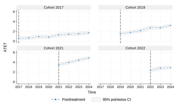
We can also obtain moderating effects. These effects tell us how the ATET changes with covariates. We believe that fines will decrease the effect of hoverboards on accidents. We obtain
. estat moderation

Moderating effects                                       Number of obs = 4,320

                                   (Std. err. adjusted for 432 clusters in id)
| Robust | ||
| Effect std. err. z P>|z| [95% conf. interval] | ||
| fines | ||
| _did_cohort# | ||
| year | ||
| 2017 2017 | -.6368641 .4691538 -1.36 0.175 -1.556389 .2826605 | |
| 2017 2018 | -.6152899 .3126822 -1.97 0.049 -1.228136 -.0024441 | |
| 2017 2019 | -.624898 .3227653 -1.94 0.053 -1.257506 .0077104 | |
| 2017 2020 | -.8951207 .3652096 -2.45 0.014 -1.610918 -.179323 | |
| 2017 2021 | -1.066773 .408465 -2.61 0.009 -1.86735 -.2661967 | |
| 2017 2022 | -.5156622 .4607561 -1.12 0.263 -1.418727 .3874031 | |
| 2017 2023 | -.6859404 .4659089 -1.47 0.141 -1.599105 .2272243 | |
| 2017 2024 | -.567364 .3774481 -1.50 0.133 -1.307149 .1724206 | |
| 2019 2019 | .5211306 .4159051 1.25 0.210 -.2940285 1.33629 | |
| 2019 2020 | -.3232818 .5073197 -0.64 0.524 -1.31761 .6710466 | |
| 2019 2021 | -.7274432 .4146683 -1.75 0.079 -1.540178 .0852918 | |
| 2019 2022 | -.1822911 .3738946 -0.49 0.626 -.9151111 .5505288 | |
| 2019 2023 | -.8057648 .3736564 -2.16 0.031 -1.538118 -.0734117 | |
| 2019 2024 | -.3862243 .4149699 -0.93 0.352 -1.19955 .4271018 | |
| 2021 2021 | -1.081212 .307387 -3.52 0.000 -1.68368 -.4787447 | |
| 2021 2022 | -.951955 .3793169 -2.51 0.012 -1.695402 -.2085076 | |
| 2021 2023 | -.898084 .3248146 -2.76 0.006 -1.534709 -.261459 | |
| 2021 2024 | -1.215571 .370437 -3.28 0.001 -1.941614 -.4895277 | |
| 2022 2022 | -1.302877 .5085926 -2.56 0.010 -2.299701 -.3060541 | |
| 2022 2023 | -1.945436 .4705951 -4.13 0.000 -2.867785 -1.023087 | |
| 2022 2024 | -1.525409 .3369357 -4.53 0.000 -2.185791 -.8650273 | |
The results above confirm our suggestion. The moderating effects are negative for the 2021 and 2022 cohorts and for some periods for the other cohorts.
Read more about nonlinear heterogeneous DID in [CAUSAL] xthdidfracreg, [CAUSAL] xthdidlogit, and [CAUSAL] xthdidpoisson in the Stata Causal Inference and Treatment-Effects Estimation Reference Manual.
Learn more about Stata's causal inference features.
View all the new features in Stata 19 and, in particular, new in causal inference.


