Use the new robias() and plot() options with meta forestplot to create more informative forest plots. Display color-coded risk-of-bias (RoB) assessments alongside study results via the robias() option, or display multiple sets of effect sizes and confidence intervals side by side in the same forest plot by using the repeated plot() option. These features are part of StataNow™.

Forest plots provide a compact visual summary of study-specific effect sizes, confidence intervals, and the overall meta-analysis result. But sometimes you want to display more. Readers may want to assess the RoB of individual studies without consulting a separate table, or they may want to compare multiple estimates for each study, for example, uncorrected and corrected effect sizes or observed versus shrinkage estimates in Bayesian meta-analysis. Multiple-effect forest plots can also be useful for displaying results from bivariate or multivariate meta-analyses, where estimates for multiple outcomes or effect sizes can be presented side by side.

The new robias() option lets you add RoB assessments directly to a forest plot as color-coded columns, including a separate overall risk judgment. The new plot() option lets you add one or more sets of study-specific effect sizes and confidence intervals, each with its own plot region and x axis. And the two options can be combined to present study results, additional effect sizes, and RoB assessments in a single forest plot.

Let's see it work

The saga continues: Reviewer #2 has requests for the mindful eating book

The lentil sliders are still on the menu, and the mindful eating book is under review thanks to your psychometric meta-analysis. Just when you thought your role as the family's in-house meta-analyst was finished, reviewer #2 responds with two requests. The publisher wants a forest plot that displays formal RoB assessments for each of the 13 studies, and they also want the raw, uncorrected correlations shown alongside the corrected values from the psychometric meta-analysis.

Two requests, two new options. You already know where to start.

Fictional dataset: Preparing the RoB data

During the psychometric meta-analysis, you had already recorded RoB assessments for each study. Because these studies report correlations between mindful eating and self-control, randomized trial sources of bias (also known as RoB domain variables) such as randomization and blinding of participants are not suitable in this context. Instead, you use three domains that are more relevant for correlational studies of psychological constructs: sample selection (rob_sel), measurement quality (rob_meas), and reporting or analysis clarity (rob_report).

These RoB variables are not estimated by the meta-analysis model. They are reviewer assessments (in this case, yours) recorded during data extraction. Each domain is stored as a factor variable in the dataset, with values 1 for low risk, 2 for unclear risk, and 3 for high risk. All you need to do is label the columns.

. label variable rob_sel        "S"
. label variable rob_meas       "M"
. label variable rob_report     "R"
. label variable rob_overall    "O"

These one-letter labels are standard practice in RoB forest plots to display the domain variables compactly on the plot.

Adding RoB columns to the forest plot

The new robias() option takes a list of RoB domain variables and appends one color-coded column per variable to the right of the standard forest plot. Green circles signal low risk, orange circles signal unclear risk, and red circles signal high risk. A legend identifying the three categories appears automatically below the x axis.

. quietly meta psycorr rxyr n, xrel(rxxr) yrel(ryyr) xuratios(ux) studylabel(studylbl)
. meta forest, robias(rob_sel rob_meas rob_report)

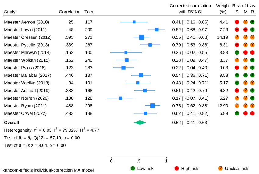
The three RoB columns on the right let readers instantly assess each study's risk level across the three sources of potential bias—no separate table required.

Separating the overall risk judgment

Reviewer #2 specifically asked for an overall RoB judgment in a column of its own, visually set apart from the domain assessments. The orisk() suboption handles this. It adds a fourth column with a thin spacer gap between the domain block and the overall judgment column.

. meta forest, robias(rob*, orisk(rob_overall) unclearlabel("Some concerns"))

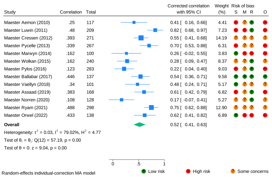
We have also specified the unclearlabel() option to change the label for the orange circles to “Some concerns” instead of the default “Unclear risk”. The gap makes the distinction between domain-level and study-level judgments clear at a glance—exactly what the reviewer was looking for.

This is the figure you attach to the revision. One request down.

Comparing observed and corrected correlations side by side

The second request—displaying the uncorrected correlations alongside the corrected ones—calls for the new plot() option. You provide the names of three variables holding the point estimate, the lower CI bound, and the upper CI bound of the observed (uncorrected) correlations, and plot() adds an extra forest graph column (_plot-like column) to the forest plot. You may use the overall() suboption to place a summary diamond (representing the overall observed correlation) at the foot of the extra forest graph, mirroring the main overall diamond corresponding to the overall corrected correlation.

First, we compute all the necessary components to feed into the plot() option. These consist of the study-specific observed correlations (rxyr) and their CIs (cil and ciu) and the overall observed correlation and its CI (stored in scalars theta, ci_ub, and ci_lb, respectively).

. quietly meta esize rxyr n, esize(correlation) studylabel(studylbl)
. clonevar cil = _meta_cil
. clonevar ciu = _meta_ciu

. quietly meta summarize
. scalar theta = r(theta)
. scalar ci_ub = r(ci_ub)
. scalar ci_lb = r(ci_lb)

Without artifact correction, the pooled correlation across the 13 studies is 0.32. Next, we will show these observed correlations on the forest plot as an additional forest graph before the _plot column corresponding to the corrected correlations.

. qui meta psycorr rxyr n, xrel(rxxr) yrel(ryyr) xuratios(ux) studylabel(studylbl )
. meta forest,  esrefline robias(rob_sel rob_meas rob_report,
    orisk(rob_overall) unclearlabel("Some concerns"))
    plot(rxyr cil ciu, before(_plot) title("Observed correlation")
    overall(`=theta' `=ci_lb' `=ci_ub') xline(`=theta'))
    columnopts(_plot, title("Corrected correlation"))
    

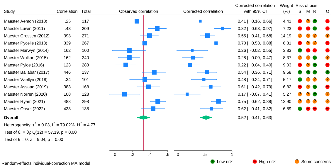
The gap between the two summary diamonds—0.32 versus 0.518—makes the case for psychometric correction more convincingly than any table could.

Reviewer #2 is satisfied with how you handled his requests. Your future mother-in-law frames the acceptance letter and hangs it next to the lentil slider recipe.