1 item has been added to your cart.
You may be interested in Bayesian analysis if
Overview of Bayesian analysis.
Stata 14 provides a new suite of features for performing Bayesian analysis. Stata's bayesmh fits a variety of Bayesian regression models using an adaptive Metropolis–Hastings (MH) Markov chain Monte Carlo (MCMC) method. Gibbs sampling is also supported for selected likelihood and prior combinations. Commands for checking convergence and efficiency of MCMC, for obtaining posterior summaries for parameters and functions of parameters, for hypothesis testing, and for model comparison are also provided.
Your Bayesian analysis can be as simple or as complicated as your research problem. Here's an overview.
Suppose we want to estimate the mean car mileage mpg. Our standard frequentist analysis may fit a regression model to mpg and look at the constant _cons.
. regress mpg
| Source | SS df MS | Number of obs = 74 | |
| F(0, 73) = 0.00 | |||
| Model | 0 0 . | Prob > F = . | |
| Residual | 2443.45946 73 33.4720474 | R-squared = 0.0000 | |
| Adj R-squared = 0.0000 | |||
| Total | 2443.45946 73 33.4720474 | Root MSE = 5.7855 |
| mpg | Coef. Std. Err. t P>|t| [95% Conf. Interval] | |
| _cons | 21.2973 .6725511 31.67 0.000 19.9569 22.63769 | |
To fit a Bayesian model, in addition to specifying a distribution or a likelihood model for the outcome of interest, we must also specify prior distributions for all model parameters.
For simplicity, let's model mpg using a normal distribution with a known variance of, say, 35 and use a noninformative flat prior (with a density of 1) for the mean parameter {mpg:_cons}.
. bayesmh mpg, likelihood(normal(35)) prior({mpg:_cons}, flat)

Burn-in ...
Simulation ...

Model summary
| Likelihood: |
| mpg ~ normal({mpg:_cons},35) |
| Prior: |
| {mpg:_cons} ~ 1 (flat) |
| Equal-tailed | ||
| mpg | Mean Std. Dev. MCSE Median [95% Cred. Interval] | |
| _cons | 21.30713 .6933058 .015564 21.32559 19.91967 22.64948 | |
bayesmh discarded the first 2,500 burn-in iterations and used the subsequent 10,000 MCMC iterations to produce the results. The estimated posterior mean, the mean of the posterior distribution, of parameter {mpg:_cons} is close to the OLS estimate obtained earlier, as is expected with the noninformative prior. The estimated posterior standard deviation is close to the standard error of the OLS estimate.
The MCSE of the posterior mean estimate is 0.016. The MCSE is about the accuracy of our simulation results. We would like it to be zero, but that would take an infinite number of MCMC iterations. We used 10,000 iterations and have results accurate to about 1 decimal place. That's good enough, but if we wanted more accuracy, we could increase the MCMC sample size.
According to the credible interval, the probability that the mean of mpg is between 19.92 and 22.65 is about 0.95. Although the confidence interval reported on our earlier regression has similar values, it does not have the same probabilistic interpretation.
Because bayesmh uses MCMC, a simulation-based method, the results will be different every time we run the command. (Inferential conclusions should stay the same provided MCMC converged.) You may want to specify a random-number seed for reproducibility in your analysis.
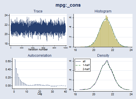
The interpretation of our results is valid only if MCMC converged. Let's explore convergence visually.
. bayesgraph diagnostics {mpg:_cons}, histopts(normal)

The trace plot of {mpg:_cons} demonstrates good mixing. The autocorrelation dies off quickly. The posterior distribution of {mpg:_cons} resembles the normal distribution, as is expected for the specified likelihood and prior distributions. We have no reason to suspect nonconvergence.
We can now proceed with further analysis.
We can test an interval hypothesis that the mean mileage is greater than 21.
. bayestest interval {mpg:_cons}, lower(21)

Interval tests     MCMC sample size =    10,000

       prob1 : {mpg:_cons} > 21
| Mean Std. Dev. MCSE | ||
| prob1 | .6735 0.46896 .0099939 | |
The estimated probability of this interval hypothesis is 0.67. This is in contrast with the classical hypothesis testing that provides a deterministic decision of whether to reject the null hypothesis that the mean is greater than 21 based on some prespecified level of significance. Frequentist hypothesis testing does not assign probabilistic statements to the tested hypotheses.
Suppose that based on previous studies, we have prior information that the mean mileage is normally distributed with mean 30 and variance 5. We can easily incorporate this prior information in our Bayesian model. We will also store our MCMC and estimation results for future comparison.
. bayesmh mpg, likelihood(normal(35)) prior({mpg:_cons}, normal(30,5))
              saving(prior1_sim)

Burn-in ...
Simulation ...

Model summary
| Likelihood: |
| mpg ~ normal({mpg:_cons},35) |
| Prior: |
| {mpg:_cons} ~ normal(30,5) |
| Equal-tailed | ||
| mpg | Mean Std. Dev. MCSE Median [95% Cred. Interval] | |
| _cons | 22.0617 .6683529 .014619 22.05628 20.75121 23.39481 | |
This prior resulted in a slight increase of the posterior mean estimate—the prior shifted the estimate toward the specified prior mean of 30.
Suppose that another competing prior is that the mean mileage is normally distributed with mean 20 and variance 4.
. bayesmh mpg, likelihood(normal(35)) prior({mpg:_cons}, normal(20,4))
              saving(prior2_sim)

Burn-in ...
Simulation ...

Model summary
| Likelihood: |
| mpg ~ normal({mpg:_cons},35) |
| Prior: |
| {mpg:_cons} ~ normal(20,4) |
| Equal-tailed | ||
| mpg | Mean Std. Dev. MCSE Median [95% Cred. Interval] | |
| _cons | 21.17991 .6658923 .014733 21.17731 19.87617 22.47459 | |
The results using this prior are more similar to the earlier results with the noninformative prior.
We can compare our two models that used different informative priors. Estimation results of the models were stored under prior1 and prior2. To compare the models, we type
. bayesstats ic prior1 prior2

Bayesian information criteria
| DIC log(ML) log(BF) | ||
| prior1 | 472.0359 -242.5827 . | |
| prior2 | 470.8157 -235.7438 6.838942 | |
The second model has a lower DIC value and is thus preferable.
Bayes factors—log(BF)—are discussed in [BAYES] bayesstats ic. All we will say here is that the value of 6.84 provides very strong evidence in favor of our second model, prior2.
We can also compute posterior probabilities for each model.
. bayestest model prior1 prior2

Bayesian model tests
| log(ML) P(M) P(M|y) | ||
| prior1 | -242.5827 0.5000 0.0011 | |
| prior2 | -235.7438 0.5000 0.9989 | |
The posterior probability of the first model is very low compared with that of the second model. In fact, the posterior probability of the first model is near 0, whereas the posterior probability of the second model is near 1.
Continuing our car-mileage example, we now relax the assumption of a known variance of the normal distribution and model it as a parameter {var}. We specify a noninformative Jeffreys prior for the variance parameter.
. bayesmh mpg, likelihood(normal({var})) prior({mpg:_cons}, flat)
                                         prior({var}, jeffreys)

Burn-in ...
Simulation ...

Model summary
| Likelihood: |
| mpg ~ normal({mpg:_cons},{var}) |
| Priors: |
| {mpg:_cons} ~ 1 (flat) |
| {var} ~ jeffreys |
| Equal-tailed | ||
| Mean Std. Dev. MCSE Median [95% Cred. Interval] | ||
| mpg | ||
| _cons | 21.30678 .7018585 .023602 21.30086 19.91435 22.72222 | |
| var | 34.38441 5.787753 .149506 33.73722 24.71946 47.7112 | |
Note that the MCSE for parameter {mpg:_cons} is larger in this model than it was in the model with a fixed variance. As the number of model parameters increases, the efficiency of the MH algorithm decreases, and the task of constructing an efficient algorithm becomes more and more important. In the above, for example, we could have improved the efficiency of MH by specifying the variance parameter in a separate block, block({var}), to be sampled independently of the mean parameter.
Even without adding the blocking, convergence diagnostics for both mean and variance look good.
. bayesgraph diagnostics _all


We can compute summaries for linear and nonlinear expressions of our parameters. Let's compute summaries for a standardized mean, which is a function of both the mean parameter and the variance parameter.
. bayesstats summary (mean_std: {mpg:_cons}/sqrt({var}))

Posterior summary statistics                      MCMC sample size =    10,000

    mean_std : {mpg:_cons}/sqrt({var})
| Equal-tailed | ||
| Mean Std. Dev. MCSE Median [95% Cred. Interval] | ||
| mean_std | 3.670299 .3183261 .008546 3.661119 3.060899 4.308195 | |
bayesmh makes it easy to include explanatory variables in our Bayesian models. The syntax for regressions looks just as it does in other Stata estimation commands. For example, we can include an indicator of whether the car is foreign or domestic when modeling the mean car mileage.
. bayesmh mpg foreign, likelihood(normal({var}))
                       prior({mpg:_cons foreign}, flat)
                       prior({var}, jeffreys)

Burn-in ...
Simulation ...

Model summary
| Likelihood: |
| mpg ~ normal(xb_mpg,{var}) |
| Priors: |
| {mpg:foreign _cons} ~ 1 (flat) (1) |
| {var} ~ jeffreys |
| Equal-tailed | ||
| Mean Std. Dev. MCSE Median [95% Cred. Interval] | ||
| mpg | ||
| foreign | 4.987455 1.43297 .054471 5.014443 2.034135 7.775843 | |
| _cons | 19.81477 .7796195 .030952 19.79542 18.27116 21.35802 | |
| var | 29.52163 5.304377 .194809 28.82301 20.82704 41.50129 | |
We specified a flat prior for both the constant and the coefficient of foreign.
We can fit a multivariate normal regression to model two size characteristics of automobiles, —trunk space, trunk, and turn circle, turn,— as a function of where the car is manufactured, foreign, foreign or domestic. The syntax for the regression part of the model is just like the syntax for Stata's mvreg (multivariate regression) command.
We model the covariance matrix of trunk and turn as the matrix parameter {Sigma,matrix}. We specify noninformative normal priors with large variances for all regression coefficients and use Jeffreys prior for the covariance. The MH algorithm has very low efficiencies for sampling covariance matrices, so we use Gibbs sampling instead. The regression coefficients are sampled by using the MH method.
. bayesmh trunk turn = foreign, likelihood(mvnormal({Sigma, matrix}))
                                prior({trunk:} {turn:}, normal(0,1000))
                                prior({Sigma, matrix}, jeffreys(2))
                                block({Sigma, matrix}, gibbs)

Burn-in ...
Simulation ...

Model summary
| Likelihood: |
| trunk turn ~ mvnormal(2,xb_trunk,xb_turn,{Sigma,m}) |
| Priors: |
| {trunk:foreign _cons} ~ normal(0,1000) (1) |
| {turn:foreign _cons} ~ normal(0,1000) (2) |
| {Sigma,m} ~ jeffreys(2) |
| Equal-tailed | ||
| Mean Std. Dev. MCSE Median [95% Cred. Interval] | ||
| trunk | ||
| foreign | -3.348432 1.056294 .046491 -3.337957 -5.417821 -1.375893 | |
| _cons | 14.75301 .5450302 .019877 14.73202 13.73661 15.89116 | |
| turn | ||
| foreign | -6.004471 .8822641 .038093 -5.991697 -7.751608 -4.267331 | |
| _cons | 41.42375 .4817673 .017979 41.42091 40.48585 42.42505 | |
| Sigma_1_1 | 17.11048 3.028132 .036471 16.77325 12.21387 23.93075 | |
| Sigma_2_1 | 7.583515 2.026102 .024179 7.39855 4.153189 12.07798 | |
| Sigma_2_2 | 12.537 2.175963 .024705 12.29787 9.014795 17.45602 | |
Watch how to fit this model using the GUI.
As an example of a nonlinear model, we consider a change-point analysis of the British coal-mining disaster dataset for the period of 1851 to 1962. This example is adapted from Carlin, Gelfand, and Smith (1992). In these data, the count variable records the number of disasters involving 10 or more deaths.
The graph below suggests a fairly abrupt decrease in the rate of disasters around the 1887–1895 period.

Let's estimate the date when the rate of disasters changed.
We will fit the model
count ~ Poisson(mu1), if year < cp
count ~ Poisson(mu2), if year >= cp
cp—the change point—is the main parameter of interest.
We will use noninformative priors for the parameters: flat priors for the means and a uniform on [1851,1962] for the change point.
We will model the mean of the Poisson distribution as a mixture of mu1 and mu2.
. bayesmh count, likelihood(dpoisson({mu1}*sign(year<{cp})+{mu2}*sign(year>={cp})))
                 prior({mu1 mu2}, flat)
                 prior({cp}, uniform(1851,1962))
                 initial({mu1 mu2} 1 {cp} 1906)

Burn-in ...
Simulation ...

Model summary
| Likelihood: |
| count ~ poisson({mu1}*sign(year<{cp})+{mu2}*sign(year>={cp})) |
| Hyperpriors: |
| {mu1 mu2} ~ 1 (flat) |
| {cp} ~ uniform(1851,1962) |
| Equal-tailed | ||
| Mean Std. Dev. MCSE Median [95% Cred. Interval] | ||
| mu1 | 3.118753 .3001234 .015504 3.110907 2.545246 3.72073 | |
| cp | 1890.362 2.4808 .071835 1890.553 1886.065 1896.365 | |
| mu2 | .9550596 .1209208 .005628 .9560248 .7311639 1.219045 | |
The change point is estimated to have occurred in 1890 with the corresponding 95% CrI of [1886,1896].
We may also be interested in estimating the ratio between the two means.
. bayesstats summary (ratio: {mu1}/{mu2})

Posterior summary statistics                      MCMC sample size =    10,000

       ratio : {mu1}/{mu2}
| Equal-tailed | ||
| Mean Std. Dev. MCSE Median [95% Cred. Interval] | ||
| ratio | 3.316399 .5179103 .027848 3.270496 2.404047 4.414975 | |
After 1890, the mean number of disasters decreased by a factor of about 3.3 with a 95% credible range of [2.4, 4.4].
The interpretation of our change-point results is valid only if MCMC converged. We can explore convergence visually.
. bayesgraph diagnostics {cp} (ratio: {mu1}/{mu2})


The graphical diagnostics for {cp} and the ratio look reasonable. The marginal posterior distribution of the change point has the main peak at about 1890 and two smaller bumps around the years 1886 and 1896, which correspond to local peaks in the number of disasters.
In Multivariate linear regression, we showed you how to use the command line to fit a Bayesian multivariate regression. Watch Graphical user interface for Bayesian analysis to see how to fit this model and more using the GUI.
Carlin, B. P., A. E. Gelfand, and A. F. M. Smith. 1992. Hierarchical Bayesian analysis of changepoint problems. Journal of the Royal Statistical Society, Series C 41: 389–405.
Stata's new Bayesian analysis features are documented in their own new 255-page manual. You can read more about Bayesian analysis, more about Stata's new Bayesian features, and see many worked examples in Stata Bayesian Analysis Reference Manual.
Read the overview from the Stata News and In the Spotlight: Bayesian "random effects" models.
Read the Stata Blog entries Bayesian modeling: Beyond Stata's built-in models and Gelman–Rubin convergence diagnostic using multiple chains.
Watch Bayesian analysis in Stata
Watch Introduction to Bayesian analysis, part 1: The basic concepts
Watch Introduction to Bayesian analysis, part 2: MCMC and the Metropolis-Hastings algorithm
;)