
Bayesian analysis
- Bayesian estimation
- Continuous, binary, ordered, and count outcomes
- Univariate, multivariate, and multiple-equation models
- Linear models, nonlinear models, and generalized nonlinear models
- 10 likelihood models, including univariate and multivariate normal, logit, probit, ordered logit, ordered probit, Poisson ...
- 18 prior distributions, including normal, lognormal, multivariate
normal, gamma, beta, Wishart ... - Specialized priors, such as flat, Jeffreys, and Zellner's g
- User-defined likelihoods and priors
- Or write your own programs to calculate likelihood function and
choose built-in priors - Or write your own programs to calculate posterior density directly
- MCMC methods
- Adaptive Metropolis–Hastings (MH)
- Adaptive MH with Gibbs updates
- Full Gibbs sampling for certain likelihood and prior combinations
- Graphical tools to check MCMC convergence visually
- Explore MCMC efficiency by computing effective sample sizes,
autocorrelation times, and efficiencies
- Bayesian summaries
- Posterior means and SDs
- Monte Carlo standard errors (MCSEs)
- Credible intervals (CrIs)
- Compute any of the above for parameters or functions
of parameters
- Hypothesis testing
- Interval-hypothesis testing for parameters or functions
of parameters - Model-based hypothesis testing by computing model
posterior probabilities
- Interval-hypothesis testing for parameters or functions
- Model comparison
- Bayesian information criteria such as deviance information criterion
- Bayes factors
- Save your MCMC and estimation results for future use
Your Bayesian analysis can be as simple or as complicated as your research problem. Here's an overview.
First, fit the model. If we wanted to estimate the mean cholesterol level of children aged 5–10 whose parents have high cholesterol and if we wanted to use a normal model for cholesterol levels with noninformative priors for the parameters—flat prior for the mean and Jeffreys prior for the variance—we would type
. bayesmh chol, likelihood(normal({var}))
                prior({chol:_cons}, flat)
                prior({var}, jeffreys)
Point estimates, credible intervals, etc., are reported.
If we instead wanted to assume an informative normal prior centered at 190 mg/dL with a variance of 100, all based on previous studies, we would type
. bayesmh chol, likelihood(normal({var}))
                prior({chol:_cons}, normal(190,100))
                prior({var}, jeffreys)
Either way, convergence of MCMC and the distributions of the parameters can be explored using
. bayesgraph diagnostics {chol:_cons} {var}
We may be interested in estimating the probability that the mean cholesterol level is greater than 200 based on the current sample.
. bayestest interval {chol:_cons}, lower(200)
What is Bayesian analysis
Bayesian analysis is a statistical analysis that answers research questions about unknown parameters using probability statements. For example, what is the probability that the average male height is between 70 and 80 inches or that the average female height is between 60 and 70 inches? Or, what is the probability that people in a particular state vote Republican or vote Democrat? Or, what is the probability that a person accused of a crime is guilty?
Such probabilistic statements are natural to Bayesian analysis because of the underlying assumption that all parameters are random quantities. In Bayesian analysis, a parameter is summarized by an entire distribution of values instead of the one fixed value used in classical frequentist analysis. The estimation of this distribution, the posterior distribution of a parameter of interest, is at the heart of Bayesian analysis.
Change point analysis
As an example, let's look at the British coal mining disaster dataset (1851–1962). Variable count records the number of disasters involving 10 or more deaths. There was a fairly abrupt decrease in the rate of disasters around 1887–1895. Let's estimate the date when the rate of disasters changed.
We will fit the model
count ~ Poisson(μ1), if year < cp
count ~ Poisson(μ2), if year >= cp
cp—the change point—is the main parameter of interest. We are doing what's called a change-point analysis.
We will use noninformative priors for the parameters: flat priors for the means and a uniform on [1851,1962] for the change point.
We will model the mean of the Poisson distribution as a mixture of μ1 and μ2.
To fit the model, we type
. bayesmh count, likelihood(dpoisson({mu1}*sign(year < {cp}) +
                 {mu2}*sign(year >= {cp})))
                 prior({mu1 mu2}, flat)
                 prior({cp}, uniform(1851,1962))
                 initial({mu1 mu2} 1 {cp} 1906)
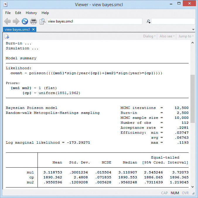
The posterior mean estimate of the change point is 1890.
The standard error of the posterior mean estimate (MCSE) is 0.07. The MCSE is about the accuracy of our simulation results. We would like it to be zero, but that would take an infinite number of MCMC iterations. We used 10,000 and have results accurate to about one decimal place. That's good enough, but if we wanted more accuracy, we could increase the MCMC sample size.
The corresponding 95% CrI of cp is [1886, 1896]. The probability that the change point is between 1886 and 1896 is about 0.95.
Next
The interpretation of our change-point results is valid only if MCMC converged. We can explore convergence visually for cp.
. bayesgraph diagnostics {cp}
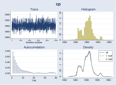
The graphical diagnostics look reasonable. The marginal posterior distribution of the change point has the main peak at about 1890 and two smaller bumps around the years 1886 and 1896, which correspond to local peaks in the number of disasters.
Change-point analysis—follow on
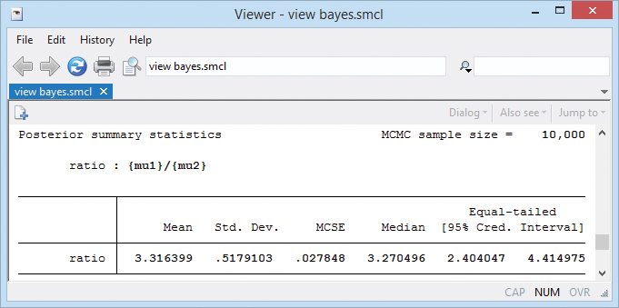
We might be interested in estimating the ratio between the two means. If we were, it would be easy to get:
. bayesstats summary (ratio: {mu1}/{mu2})
Upgrade now Order Stata Read even more about Bayesian analysis.


