← See Stata 19's new features
Highlights
Causal mediation with sequential or parallel mediators
Finest possible decomposition into path-specific effects
Coarser decomposition and mediator-specific effects
Direct effects, indirect effects, total effect, potential-outcome means, and controlled direct effects
Support for several types of interaction effects
Binary and continuous treatments
Sequential mediation sensitivity analysis
See more causal inference features
The mediate command now allows you to perform causal mediation analysis with two mediators, whether they are sequential or parallel. Estimate natural indirect effects, natural direct effects, and controlled direct effects. Obtain mediator-specific effects. Perform sensitivity analysis with sequential mediators. This feature is a part of StataNow™.
Causal mediation analysis goes beyond estimating a causal effect to exploring how the effect may arise. Is the effect of a treatment on an outcome mediated through other variables?
In Stata 18, we introduced the mediate command for fitting causal mediation models with one mediator. Now, mediate can also fit causal mediation models with two mediators. These mediators can be causally ordered (sequential) or not causally ordered (parallel). In either case, you can estimate the total effect and see how it can be decomposed into direct and indirect effects.
Suppose we wish to find out whether arthritis in humans affects their health-related quality of life. To the extent that it does, we also wish to disentangle the causal pathways through which this effect operates. In particular, we are interested in determining whether physical activity and depression mediate this effect. Does arthritis decrease physical activity, which in turn decreases quality of life? Does arthritis increase severity of depression, which in turn decreases quality of life?
To evaluate these potential mediating effects, We use fictional data including the health-related quality-of-life outcome variable (hrqol), mediator variables physical activity (physact) and depression (depress), and the binary treatment variable arthritis (arthritis). Ignoring potentially confounding variables, we can draw a causal diagram to represent our basic model:
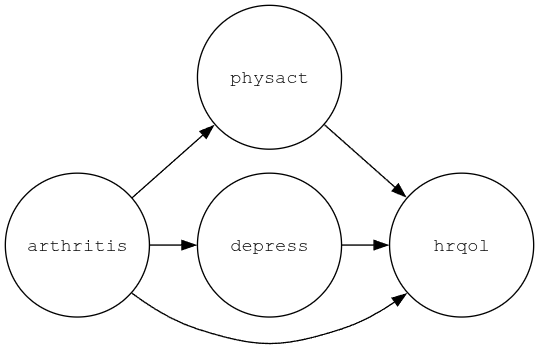
There are three causal pathways of interest: a direct pathway from arthritis to hrqol, an indirect path from arthritis to hrqol via physact, and an indirect path from arthritis to hrqol via depress. Our goal is to decompose the total causal effect of arthritis on hrqol into these three path-specific components. Because there is no causal path that goes through both mediators, we refer to these mediators as parallel.
Starting with a simple model that does not include covariates or any interaction effects, we specify the following causal mediation model:
. mediate (hrqol) (depress) (physact) (arthritis)

Iteration 0:  EE criterion = 1.537e-27
Iteration 1:  EE criterion = 8.303e-30

Causal mediation analysis                                Number of obs = 2,000

Mediation type: Parallel
Mediator 1:     physact
Mediator 2:     depress
Treatment type: Binary
| Robust | ||
| hrqol | Coefficient std. err. z P>|z| [95% conf. interval] | |
| NDE | ||
| arthritis | ||
| (Yes vs No) | -1.71165 .1496673 -11.44 0.000 -2.004993 -1.418308 | |
| NIE1 | ||
| arthritis | ||
| (Yes vs No) | -1.814969 .1817366 -9.99 0.000 -2.171166 -1.458772 | |
| NIE2 | ||
| arthritis | ||
| (Yes vs No) | -1.252368 .2507925 -4.99 0.000 -1.743912 -.7608239 | |
| TE | ||
| arthritis | ||
| (Yes vs No) | -4.778988 .2912224 -16.41 0.000 -5.349773 -4.208202 | |
The estimated total effect (TE) is −4.8 points on our (arbitrary) health-related quality-of-life scale. This effect is interpreted just like an average treatment effect: if every individual in the population had arthritis, the population average health-related quality of life score would be 5 points lower than if no one in the population had arthritis. In other words, arthritis causes a 5-point decrease in health-related quality of life, on average. The remaining estimates are the natural indirect effects (NIEs) and natural direct effect (NDE). They tell us how much of this 5-point difference is due to physical activity (NIE1), how much to depression (NIE2), and how much to neither physical activity nor depressive symptoms (NDE). The NIE1 estimate is −1.8, so almost two points of the 5-point difference are due to decreased physical activity. The indirect effect of arthritis on hrqol through depress (NIE2) is −1.3. Finally, the estimated NDE indicates that 1.7 points of the 5-point difference are due to mechanisms other than physical activity and depression.
The model above is somewhat restrictive in the sense that we apply strictly linear equations without interactions among treatment and mediators. In the single-mediator case, including a treatment–mediator interaction yields two sets of effect estimands, pure and total natural effects, resulting in two different decompositions of the total effect. Using two mediators with a parallel mediation design, however, yields a total of six decompositions and can yield as many as four estimands per effect of interest.
In the following model, we include interactions as well as covariates. We suspect that age is a confounder of the treatment–outcome and the mediator–outcome relationships, so we include age in the model for hrqol. To allow the effect of age on the outcome to vary as a function of the two mediators, we also include interaction terms by using factor-variable notation (c.depress#c.age c.physact#c.age). Finally, to allow for treatment–mediator and mediator–mediator interactions, we specify the tinteraction and minteraction options.
. mediate (hrqol age c.depress#c.age c.physact#c.age)
           (depress i.male)
	   (physact i.male)
	   (arthritis), tinteraction minteraction

Iteration 0:  EE criterion = 1.762e-25
Iteration 1:  EE criterion = 8.149e-30

Causal mediation analysis                                Number of obs = 2,000

Mediation type: Parallel
Mediator 1:     physact
Mediator 2:     depress
Treatment type: Binary
| Robust | ||
| hrqol | Coefficient std. err. z P>|z| [95% conf. interval] | |
| NDE | ||
| 00 | -2.93327 .0986156 -29.74 0.000 -3.126553 -2.739987 | |
| 10 | -2.2664 .1321111 -17.16 0.000 -2.525333 -2.007467 | |
| 01 | -3.13574 .1548724 -20.25 0.000 -3.439284 -2.832196 | |
| 11 | -2.441183 .0633247 -38.55 0.000 -2.565297 -2.317068 | |
| NIE1 | ||
| 00 | -2.559244 .2330217 -10.98 0.000 -3.015958 -2.102529 | |
| 10 | -1.892373 .1842448 -10.27 0.000 -2.253486 -1.53126 | |
| 01 | -2.596165 .2396821 -10.83 0.000 -3.065933 -2.126396 | |
| 11 | -1.901607 .1889659 -10.06 0.000 -2.271974 -1.531241 | |
| NIE2 | ||
| 00 | -.4994956 .0965284 -5.17 0.000 -.6886879 -.3103033 | |
| 10 | -.7019653 .1137533 -6.17 0.000 -.9249177 -.4790128 | |
| 01 | -.5364167 .0960709 -5.58 0.000 -.7247123 -.3481211 | |
| 11 | -.7111994 .1138654 -6.25 0.000 -.9343716 -.4880273 | |
| TE | ||
| arthritis | ||
| (Yes vs No) | -5.536843 .2526692 -21.91 0.000 -6.032065 -5.04162 | |
We now have four NDEs and four of each NIE! The effects are now referred to by an index, for example, NDE-00 or NIE1-11. Each of the effects is defined as the difference in two potential-outcome means, and these indices correspond to the counterfactual treatment levels for the potential outcomes. For example, the estimated NDE labeled 00 is −2.9 and is the natural direct effect when both of the mediators are at their values associated with no treatment (arthritis = 0). The NDEs range from −2.3 to −3.1, while the NIEs via physact range from −1.9 to −2.6, and the NIEs via depress range from −0.5 to −0.7. How much variation there is among each type of effect depends on the size of the interaction effects. In this case, while we do see variation, we still find that the largest effects are those mediated via physact (NIE1) and the direct effects (NDE).
In the two examples above, our causal model was specified such that there was no causal relation between the two mediators. Continuing with the quality-of-life data, we could instead hypothesize that physical activity causes a reduction in depression. Accounting for this causal ordering, we can draw a causal diagram that contains the additional path from physact to depress:
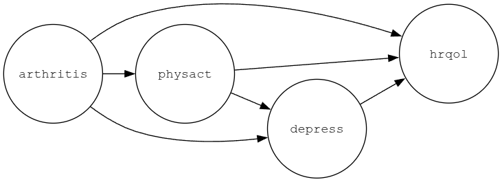
Because we have a causal path from one mediator to the other, we refer to this model as a sequential mediation model. Now there are four path-specific effects of interest: one mediated through physact alone, one mediated through depress alone, one mediated through both physact and depress, and one not mediated by either physact or depress. Let's first fit a simple variation of this model model with no interaction terms. We specify the sequential option to tell mediate that we wish to fit a sequential model. We indicate the causal order of the mediators by specifying the causal sequence from right (treatment) to left (outcome). That is, to specify that physact affects depress, we type
. mediate (hrqol age) (depress i.male) (physact i.male) (arthritis), sequential
If we wanted the causal order reversed, we would specify
. mediate (hrqol age) (physact i.male) (depress i.male) (arthritis), sequential
As before, this model is rather restrictive because it does not include any interaction terms. To include treatment–mediator interactions in the outcome equation, we can specify the tinteraction option:
. mediate (hrqol age) (depress i.male) (physact i.male) (arthritis), sequential tinteraction
Estimating all path-specific effects in the presence of interactions results in a relatively large number of estimands that can be reduced by performing a coarser decomposition, which we could do by grouping some of the path-specific effects together. For example, suppose we were primarily interested in the indirect effect via physact. In that case, we could group together any indirect effects that go through depress, which in this case would be the paths arthritis \(\rightarrow\) depress \(\rightarrow\) hrqol and arthritis \(\rightarrow\) physact \(\rightarrow\) depress \(\rightarrow\) hrqol, and focus only on the indirect effect via physact alone. We can estimate these mediator-specific effects by specifying the mseffects(physact) option:
. mediate (hrqol age) (depress i.male) (physact i.male) (arthritis), sequential tinteraction mseffects(physact)
A practitioner might want to perform an intervention study that targets one of the causal mechanisms with the intent to improve quality of life for people with arthritis. To this end, we might ask, If we could increase the amount of individuals' physical activity, could we shrink the gap in quality of life between people with and without arthritis? To answer this sort of question, we can estimate controlled direct effects (CDEs), which capture the direct effect of the treatment on the outcome when mediators are fixed at certain population values of interest. We start by evaluating the direct effect at the means of our mediators physact and depress:
. estat cde, mvalue( (mean) physact depress)

Controlled direct effect                                 Number of obs = 2,000

Mediator variables: physact depress
Mediator values:
  physact =     2.247 (mean)
  depress = 6.2440063 (mean)
| Delta-method | ||
| CDE std. err. z P>|z| [95% conf. interval] | ||
| arthritis | ||
| (Yes vs No) | -2.603496 .0609992 -42.68 0.000 -2.723052 -2.48394 | |
The estimated CDE is −2.6, which suggests that if everyone in the population would be held at the average value of the mediators, a decrease of 2.6 in quality of life is directly due to arthritis. What would happen if we could increase the amount of physical activity to five or even eight hours per month? To answer this question, we keep mediator depress at its mean and evaluate the CDE at values of five and eight hours of physical activity:
. estat cde, mvalue( (mean) depress physact=(5 8) )

Controlled direct effect                                 Number of obs = 2,000

Mediator variables: physact depress
Mediator values:
  1._at: physact =         5
         depress = 6.2440063 (mean)
  2._at: physact =         8
         depress = 6.2440063 (mean)
| Delta-method | ||
| CDE std. err. z P>|z| [95% conf. interval] | ||
| arthritis@ | ||
| _at | ||
| (Yes vs No) | ||
| 1 | -2.73777 .1385674 -19.76 0.000 -3.009357 -2.466183 | |
| (Yes vs No) | ||
| 2 | -2.884092 .2578233 -11.19 0.000 -3.389416 -2.378767 | |
The results show that if everyone in the population were to have 5 hours of physical activity (and an average depression score), the difference in quality of life due to arthritis would still be around −2.7 and not much different from the above result where physact was held at its average of 2.247. Similarly, for 8 hours of physical activity, the CDE is −2.9. Using the contrast option, we can obtain a difference between the two as well as a test:
. estat cde, mvalue( (mean) depress physact=(5 8) ) contrast

Controlled direct effect                                 Number of obs = 2,000

Mediator variables: physact depress
Mediator values:
  1._at: physact =         5
         depress = 6.2440063 (mean)
  2._at: physact =         8
         depress = 6.2440063 (mean)
| Delta-method | ||
| CDE std. err. z P>|z| [95% conf. interval] | ||
| _at# | ||
| arthritis | ||
| (2 vs 1) | ||
| (Yes vs No) | -.1463215 .1259133 -1.16 0.245 -.3931072 .1004641 | |
The difference is close to zero, which suggests that physical activity increases quality of life but does not increase it more for people with arthritis. In other words, the intervention could be helpful for all individuals but would not close the gap in quality of life between people with and without arthritis.
Read more about causal mediation analysis with two mediators in [CAUSAL] mediation multiple in the Stata Causal Inference and Treatment-Effects Estimation Reference Manual.
Learn more about Stata's causal inference features.
View all the new features in Stata 19 and, in particular, new in causal inference.


