1 item has been added to your cart.

Endogenous treatment effects were introduced in Stata 13.

See the latest version of treatment effects for endogenous treatments. See all of Stata's treatment effects features.

See the new features in Stata 18.

Endogenous treatment effects

Order

Highlights

• Relaxes conditional independence
  • Correlated unobservables that affect treatment and outcome
  • Selection on unobservables
• Estimators
  • Linear regression
  • Poisson regression
• Robust SEs to relax distributional assumptions
• Cluster–robust SEs to allow for correlated data
• Predictions
  • Potential-outcome means
  • Observed-outcome means
  • Conditional treatment effects
  • Probability of count and count-ranges for Poisson

Show me

Treatment effects measure the causal effect of a treatment on an outcome. Sometimes, we do not have conditional independence; that is, unobserved variables affecting both treatment and outcome. Endogenous treatment estimators address such cases.

etregress handles continuous outcome variables.

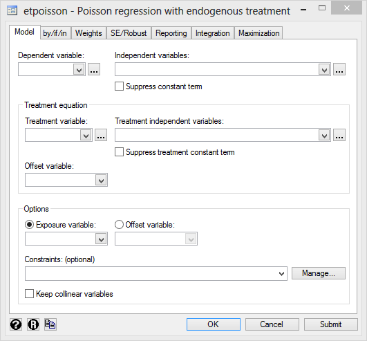
etpoisson handles count outcomes.

Suppose we are studying acne vulgaris in adults. In the data, members of the treated group have a specific genetic marker. That marker is itself determined by covariates, say, x1, x2, and x4. The outcome variable we observe is the number of pimples, and it is determined by x1 and x3. We are also concerned that there are unobserved variables that could cause the presence of the marker and affect the number of pimples.

We fit an endogenous treatment-effects model by typing

. etpoisson pustules x1 x3, treat(marker = x1 x2 x4)

Poisson regression with endogenous treatment      Number of obs   =       1000
(24 quadrature points)                            Wald chi2(3)    =      81.50
Log likelihood = -2297.3045                       Prob > chi2     =     0.0000




             
 
      Coef.   Std. Err.      z    P>|z|     [95% Conf. Interval]

 
 
 

pustules     
 
 

          x1 
 
   .0509081   .0442439     1.15   0.250    -.0358084    .1376246

          x3 
 
   .1281427   .0313078     4.09   0.000     .0667806    .1895049

    1.marker 
 
   1.329508   .1994485     6.67   0.000     .9385965     1.72042

       _cons 
 
  -.6982827   .1139443    -6.13   0.000    -.9216094   -.4749559

 
 
 

marker       
 
 

          x1 
 
   .2638588   .0469415     5.62   0.000     .1718552    .3558624

          x2 
 
  -.1921751    .048748    -3.94   0.000    -.2877194   -.0966308

          x4 
 
   .4720434   .0465768    10.13   0.000     .3807546    .5633322

       _cons 
 
  -.4946407   .1121999    -4.41   0.000    -.7145484   -.2747329

 
 
 

     /athrho 
 
   .1350499   .1706788     0.79   0.429    -.1994743    .4695742

    /lnsigma 
 
   -.285167   .0516515    -5.52   0.000     -.386402    -.183932

 
 
 

         rho 
 
   .1342348   .1676033                     -.1968701    .4378552

       sigma 
 
   .7518886   .0388361                      .6794973    .8319923


Wald test of indep. eqns. (rho = 0): chi2(1) =     0.63   Prob > chi2 = 0.4288

The output reveals no evidence of the correlation that would violate conditional independence; the point estimate of the correlation is 0.1342, and the test against 0 is insignificant.

We can obtain the average treatment effect (ATE) based on these estimates by typing

. margins r.marker

Contrasts of predictive margins
Model VCE    : OIM

Expression   : Potential-outcome mean, predict()




             
 
         df        chi2     P>chi2

 
 
 

      marker 
 
          1       28.30     0.0000





             
 
            Delta-method

             
 
   Contrast   Std. Err.     [95% Conf. Interval]

 
 
 

      marker 
 
 

   (1 vs 0)  
 
   2.584824    .485849      1.632577     3.53707

The presence of the marker adds on average 2.58 pustules.

Show me more

Read much more about endogenous treatment in the manuals at etregress and etpoisson.

Back to highlights

See New in Stata 18 to learn about what was added in Stata 18.