Table types:
One-way
Two-way
Multiway
Summary statistics
Regression comparisons
Estimation and postestimation results
Custom
Flexible table command
dtable command for easy "table one" tables
etable command for tables of regression results
System for collecting results from multiple commands and producing tables of results
Export tables to:
Word®
Excel®
HTML
LaTeX
and more
See more reporting features
Stata is ready to help you create both standard and customized tables, whether you want a table for the web that looks like
;)
or a table for your paper in Word® that looks like
;)
or that same table for your LaTeX paper
;)
You can create a lot of different tables directly using the table command—from simple cross-tabulations all the way to comparative regression tables.
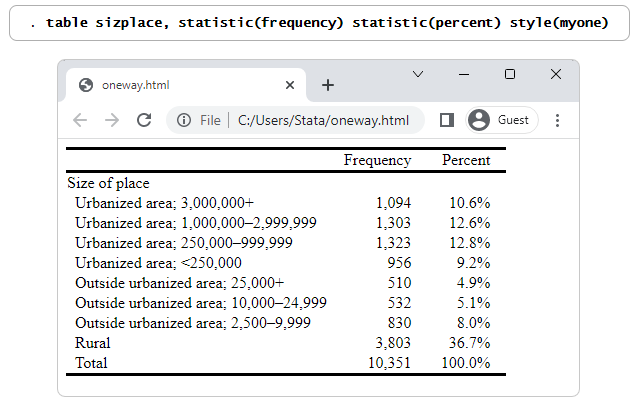
One-way frequencies and percentages
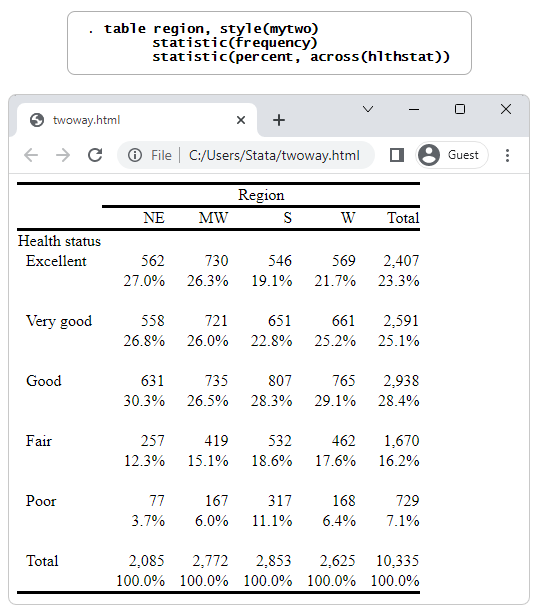
Two-way frequencies and percentages
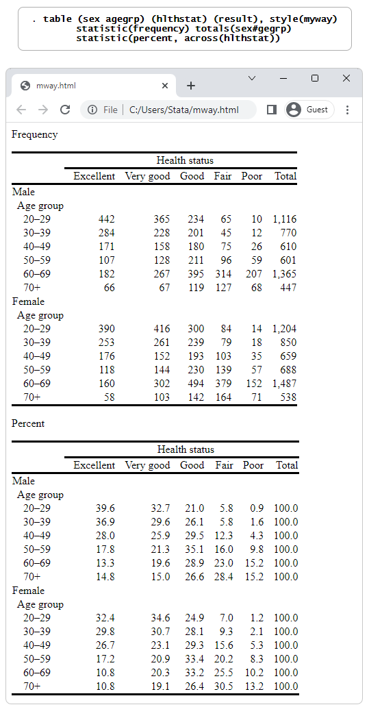
Multiway frequencies and percentages
Multiway means, SEs, frequencies, and percentages
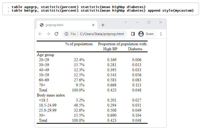
Outcome proportions
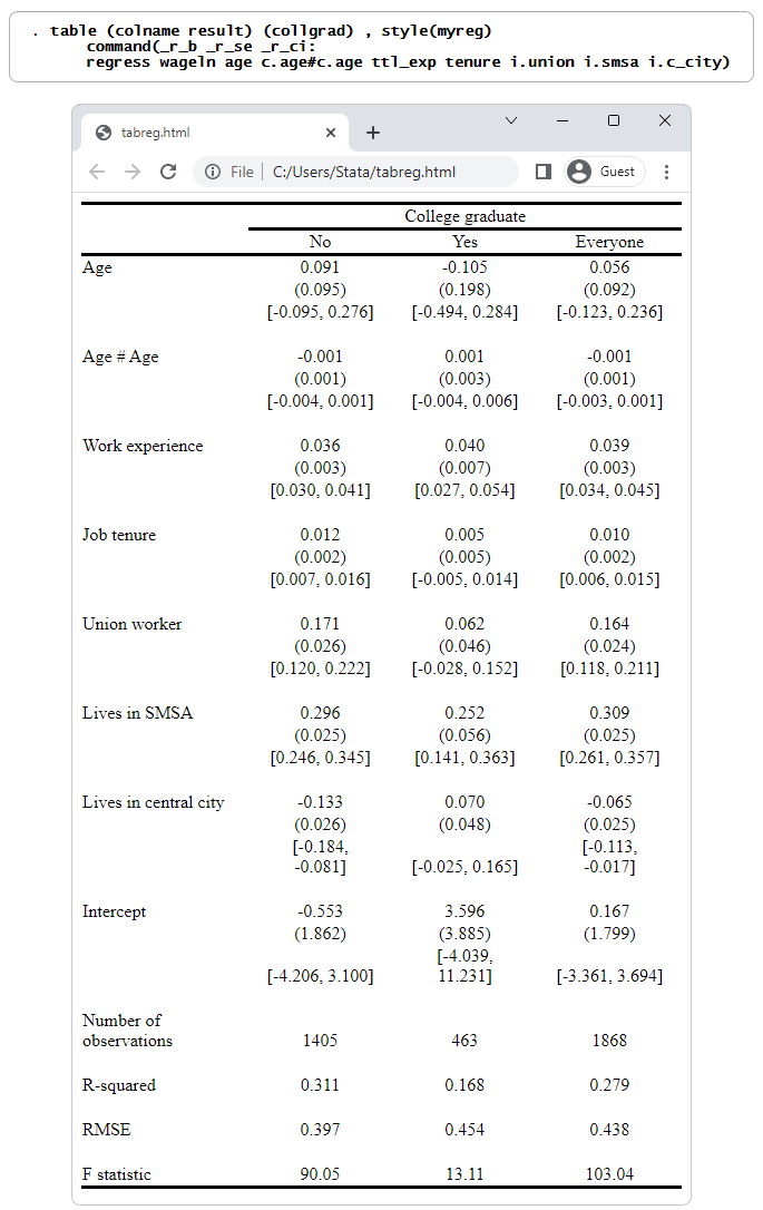
Regression comparisons
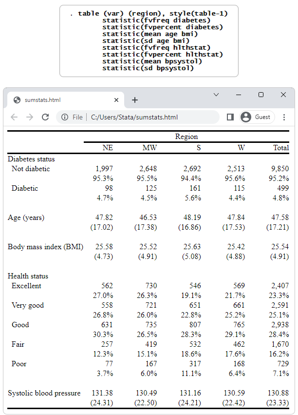
And if you are interested in summary tables for continuous and categorical variables, you can use the dtable command.
;)
;)
;)
And if you are specifically interested in creating tables of estimation results, you can use the etable command.
;)
Regression result with stars
;)
Regression comparison
;)
Regression coefficients and marginal effects
How can the table command, etable command, and the new dtable do all that? They are built on top of a whole system for collecting stored results from commands and displaying those results as tables. Stata gives you access to that system too.
We admit that the collection system harbors some complexity. One feature that makes it more approachable is styles. You saw styles being used on the table commands for the tables presented above.
You can design your own styles for the types of tables you often create. Once you have designed a style, you simply apply that style to other collected results to create a table—a table with your preferred layout, formatting, and appearance. You can also use the styles shipped with Stata or styles created by your colleagues.
Let's create a table using the collection system. We grab the NHANES II data (McDowell et al. 1981) that are used in many examples in the manuals.
. webuse nhanes2l
First, we collect the results for a simple regression of systolic blood pressure on weight in kilograms. To collect the results, all we do is place the collect prefix in front of the command:
. collect: regress bpsystol weight
Why stop with one regression? Let's add indicators for birth sex and for levels of age group to our regression. We collect those results too:
. collect: regress bpsystol weight i.sex i.agegrp
Finally, let's interact sex and age group, and collect those results:
. collect: regress bpsystol weight i.sex i.agegrp i.sex#i.agegrp
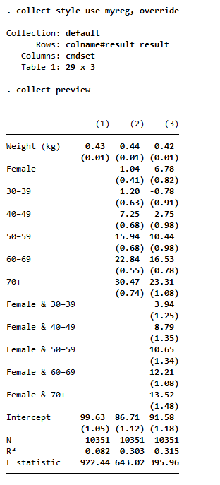
We will use a relatively simple regression style file that places the standard errors below the coefficients and adds a few model statistics to the bottom. The style's name is myreg. With a style in hand, all we do is ask the system to use that style. collect will then lay out, format, and style the table according to the specified style. We can then preview the table.
What if you prefer confidence intervals? We also have a style that shows just coefficients and confidence intervals—style myregci. We simply tell collect to use style myregci:
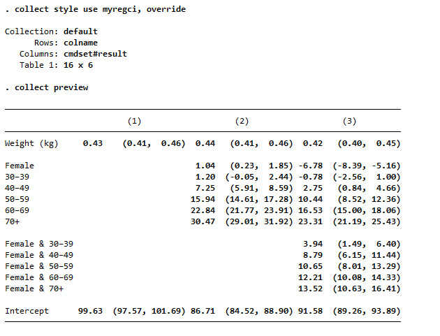
All we did to change from the first table to the second table was change the style. The two styles we applied to our collection produced distinctly different tables. The second style even puts the coefficient statistics side by side rather than above and below.
Style myregci was derived from style myreg. To create myregci from myreg, we only had to type three lines:
. collect style autolevels result _r_b _r_ci , clear
. collect style column, dups(center)
. collect layout (colname) (cmdset#result)
The first line tells collect to report only coefficients (_r_b) an confidence intervals (_r_ci). The second line tells collect how the table is to be laid out. In words, put the covariate names (colname) on the rows of the table, and put each combination of estimation command and coefficient/confidence interval on the columns (cmdset#result). The third line tells collect to center the estimation-command labels—(1), (2), and (3)—over the two columns that each label spans.
Once your table is created, you can get it into your report quickly.
Type
. collect export mytable.docx
and your table is in a file ready for Microsoft Word®.
;)
Type
. collect export mytable.html
and your table is ready for the web.
;)
Type
. collect export mytable.tex
and your table is ready to go into your LaTeX file.
;)
Here is the actual LaTeX code:
\documentclass{article}
\usepackage{multirow}
\usepackage{amsmath}
\usepackage{ulem}
\usepackage[table]{xcolor}
\begin{document}
\begin{tabular}{lllllll}
\cline{1-7}
\multicolumn{1}{c}{} &
  \multicolumn{2}{c}{(1)} &
  \multicolumn{2}{c}{(2)} &
  \multicolumn{2}{c}{(3)} \\
\cline{1-7}
\multicolumn{1}{l}{Weight (kg)} &
  \multicolumn{1}{r}{0.43 } &
  \multicolumn{1}{r}{(0.41,  0.46)} &
  \multicolumn{1}{r}{0.44 } &
  \multicolumn{1}{r}{(0.41,  0.46)} &
  \multicolumn{1}{r}{0.42 } &
  \multicolumn{1}{r}{(0.40,  0.45)} \\
\multicolumn{1}{l}{} &
  \multicolumn{1}{r}{} &
  \multicolumn{1}{r}{} &
  \multicolumn{1}{r}{} &
  \multicolumn{1}{r}{} &
  \multicolumn{1}{r}{} &
  \multicolumn{1}{r}{} \\
\multicolumn{1}{l}{Female} &
  \multicolumn{1}{r}{} &
  \multicolumn{1}{r}{} &
  \multicolumn{1}{r}{1.04 } &
  \multicolumn{1}{r}{(0.23,  1.85)} &
  \multicolumn{1}{r}{-6.78 } &
  \multicolumn{1}{r}{(-8.39, -5.16)} \\
\multicolumn{1}{l}{30-39} &
  \multicolumn{1}{r}{} &
  \multicolumn{1}{r}{} &
  \multicolumn{1}{r}{1.20 } &
  \multicolumn{1}{r}{(-0.05,  2.44)} &
  \multicolumn{1}{r}{-0.78 } &
  \multicolumn{1}{r}{(-2.56,  1.00)} \\
\multicolumn{1}{l}{40-49} &
  \multicolumn{1}{r}{} &
  \multicolumn{1}{r}{} &
  \multicolumn{1}{r}{7.25 } &
  \multicolumn{1}{r}{(5.91,  8.59)} &
  \multicolumn{1}{r}{2.75 } &
  \multicolumn{1}{r}{(0.84,  4.66)} \\
\multicolumn{1}{l}{50-59} &
  \multicolumn{1}{r}{} &
  \multicolumn{1}{r}{} &
  \multicolumn{1}{r}{15.94 } &
  \multicolumn{1}{r}{(14.61, 17.28)} &
  \multicolumn{1}{r}{10.44 } &
  \multicolumn{1}{r}{(8.52, 12.36)} \\
\multicolumn{1}{l}{60-69} &
  \multicolumn{1}{r}{} &
  \multicolumn{1}{r}{} &
  \multicolumn{1}{r}{22.84 } &
  \multicolumn{1}{r}{(21.77, 23.91)} &
  \multicolumn{1}{r}{16.53 } &
  \multicolumn{1}{r}{(15.00, 18.06)} \\
\multicolumn{1}{l}{70+} &
  \multicolumn{1}{r}{} &
  \multicolumn{1}{r}{} &
  \multicolumn{1}{r}{30.47 } &
  \multicolumn{1}{r}{(29.01, 31.92)} &
  \multicolumn{1}{r}{23.31 } &
  \multicolumn{1}{r}{(21.19, 25.43)} \\
\multicolumn{1}{l}{} &
  \multicolumn{1}{r}{} &
  \multicolumn{1}{r}{} &
  \multicolumn{1}{r}{} &
  \multicolumn{1}{r}{} &
  \multicolumn{1}{r}{} &
  \multicolumn{1}{r}{} \\
\multicolumn{1}{l}{Female \& 30-39} &
  \multicolumn{1}{r}{} &
  \multicolumn{1}{r}{} &
  \multicolumn{1}{r}{} &
  \multicolumn{1}{r}{} &
  \multicolumn{1}{r}{3.94 } &
  \multicolumn{1}{r}{(1.49,  6.40)} \\
\multicolumn{1}{l}{Female \& 40-49} &
  \multicolumn{1}{r}{} &
  \multicolumn{1}{r}{} &
  \multicolumn{1}{r}{} &
  \multicolumn{1}{r}{} &
  \multicolumn{1}{r}{8.79 } &
  \multicolumn{1}{r}{(6.15, 11.44)} \\
\multicolumn{1}{l}{Female \& 50-59} &
  \multicolumn{1}{r}{} &
  \multicolumn{1}{r}{} &
  \multicolumn{1}{r}{} &
  \multicolumn{1}{r}{} &
  \multicolumn{1}{r}{10.65 } &
  \multicolumn{1}{r}{(8.01, 13.29)} \\
\multicolumn{1}{l}{Female \& 60-69} &
  \multicolumn{1}{r}{} &
  \multicolumn{1}{r}{} &
  \multicolumn{1}{r}{} &
  \multicolumn{1}{r}{} &
  \multicolumn{1}{r}{12.21 } &
  \multicolumn{1}{r}{(10.08, 14.33)} \\
\multicolumn{1}{l}{Female \& 70+} &
  \multicolumn{1}{r}{} &
  \multicolumn{1}{r}{} &
  \multicolumn{1}{r}{} &
  \multicolumn{1}{r}{} &
  \multicolumn{1}{r}{13.52 } &
  \multicolumn{1}{r}{(10.63, 16.41)} \\
\multicolumn{1}{l}{} &
  \multicolumn{1}{r}{} &
  \multicolumn{1}{r}{} &
  \multicolumn{1}{r}{} &
  \multicolumn{1}{r}{} &
  \multicolumn{1}{r}{} &
  \multicolumn{1}{r}{} \\
\multicolumn{1}{l}{Intercept} &
  \multicolumn{1}{r}{99.63 } &
  \multicolumn{1}{r}{(97.57, 101.69)} &
  \multicolumn{1}{r}{86.71 } &
  \multicolumn{1}{r}{(84.52, 88.90)} &
  \multicolumn{1}{r}{91.58 } &
  \multicolumn{1}{r}{(89.26, 93.89)} \\
\cline{1-7}
\end{tabular}
\end{document}
You can even use the putdocx, putexcel, and putpdf systems to insert your tables directly into longer documents.
Once you have collected your results, you can work using commands to lay out, format, and style your table. Or, you can use the interactive Tables Builder.
;)
McDowell, A., A. Engel, J. T. Massey, and K. Maurer. 1981. Plan and operation of the Second National Health and Nutrition Examination Survey, 1976–1980. Vital and Health Statistics, 1(15): 1144.
You can read more about tables in the Stata Customizable Tables and Collected Results Reference Manual.
To learn more about the table command, see [R] table intro.


