Linear multilevel models

Let's see it work

Here are some examples from the mixed manual entry.

Example 1: Two-level random intercept model

Consider a longitudinal dataset used by both Ruppert, Wand, and Carroll (2003) and Diggle et al. (2002), consisting of weight measurements of 48 pigs on nine successive weeks. Pigs are identified by variable id. Below is a plot of the growth curves for the first 10 pigs.

. webuse pig
(Longitudinal analysis of pig weights)

. twoway scatter weight week if id<=10, connect(L)

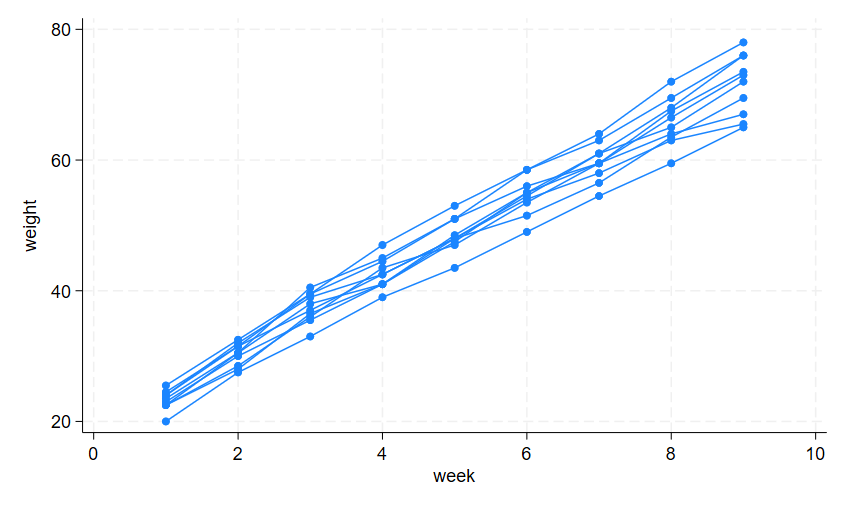
It seems clear that each pig experiences a linear trend in growth and that overall weight measurements vary from pig to pig. Because we are not really interested in these particular 48 pigs per se, we instead treat them as a random sample from a larger population and model the between-pig variability as a random effect or, equivalently, as a random-intercept term at the pig level. We thus wish to fit the following model

\(weight_{ij} = b_0 + b_1week_{ij} + u_j + e_{ij} \;\;\;\;\;\;\;\;\;\;\;\;\;\;\;\;\)(4)

for \(i\) = 1,...,9 and \(j\) = 1,...,48. The fixed portion of the model, \(b_0 + b_1week_{ij}\), simply states that we want one overall regression line representing the population average. The random effect \(u_j\) serves to shift this regression line up or down for each pig. Because the random effects occur at the pig-level, we fit the model by typing

. mixed weight week || id:

Performing EM optimization ...

Performing gradient-based optimization:
Iteration 0:  Log likelihood = -1014.9268
Iteration 1:  Log likelihood = -1014.9268

Computing standard errors ...

Mixed-effects ML regression                        Number of obs    =      432
Group variable: id                                 Number of groups =       48
                                                   Obs per group:
                                                                min =        9
                                                                avg =      9.0
                                                                max =        9
                                                   Wald chi2(1)     = 25337.49
Log likelihood = -1014.9268                        Prob > chi2      =   0.0000



      weight 
 
 Coefficient  Std. err.      z    P>|z|     [95% conf. interval]
 
 
 
        week 
 
   6.209896   .0390124   159.18   0.000     6.133433    6.286359
       _cons 
 
   19.35561   .5974059    32.40   0.000     18.18472    20.52651





  Random-effects parameters  
 
   Estimate   Std. err.     [95% conf. interval]
 
 
 
id: Identity                 
 
                  var(_cons) 
 
   14.81751   3.124225      9.801716    22.40002
 
 
 
               var(Residual) 
 
   4.383264   .3163348      3.805112     5.04926

LR test vs. linear model: chibar2(01) = 472.65        Prob >= chibar2 = 0.0000

. estimates store randint

At this point, a guided tour of the model specification and output is in order:

1. By typing weight week, we specified the response, weight, and the fixed portion of the model in the same way that we would if we were using regress or any other estimation command. Our fixed effects are a coefficient on week and a constant term.

2. When we added “|| id:”, we specified random effects at the level identified by the group variable id, that is, the pig level (level two). Because we wanted only a random intercept, that is all we had to type.

3. The estimation log consists of three parts:

1. A set of EM iterations used to refine starting values. By default, the iterations themselves are not displayed, but you can display them with the emlog option.

2. A set of gradient-based iterations. By default, these are Newton—Raphson iterations, but other methods are available by specifying the appropriate maximize options; see [R] maximize.

3. The message “Computing standard errors”. This is just to inform you that mixed has finished its iterative maximization and is now reparameterizing from a matrix-based parameterization (see Methods and formulas) to the natural metric of variance components and their estimated standard errors.

4. The output title, “Mixed-effects ML regression”, informs us that our model was fit using ML, the default. For REML estimates, use the reml option.

   Because this model is a simple random-intercept model fit by ML, it would be equivalent to using xtreg with its mle option.

5. The first estimation table reports the fixed effects. We estimate \(\beta_0\) = 19.36 and \(\beta_1\) = 6.21.

6. The second estimation table shows the estimated variance components. The first section of the table is labeled id: Identity, meaning that these are random effects at the id (pig) level and that their variance—covariance matrix is a multiple of the identity matrix; that is, \(\sum = \sigma_u^2 I\). Because we have only one random effect at this level, mixed knew that Identity is the only possible covariance structure. In any case, the variance of the level-two errors, \(\sigma_u^2\) is estimated as 14.82 with standard error 3.12.

7. The row labeled var(Residual) displays the estimated variance of the overall error term; that is, \(\hat{\sigma}^2_\epsilon\) = 4.38. This is the variance of the level-one errors, that is, the residuals.

8. Finally, a likelihood-ratio test comparing the model with one-level ordinary linear regression, model (4) without \(\mathit {u_j}\), is provided and is highly significant for these data.

   We now store our estimates for later use:

   . estimates store randint

Example 2: Two-level random slope model

Extending (4) to also allow for a random slope on week yields the model

\(weight_{ij} = b_0 + b_1week_{ij} + u_{0j} + u_{1j}week_{ij} + e_{ij} \;\;\;\;\;\;\;\;\;\;\;\;\;\;\;\;\)(5)

and we fit this with mixed.

. mixed weight week || id: week

Performing EM optimization ...

Performing gradient-based optimization:
Iteration 0:  Log likelihood = -869.03825
Iteration 1:  Log likelihood = -869.03825

Computing standard errors ...

Mixed-effects ML regression                         Number of obs    =     432
Group variable: id                                  Number of groups =      48
                                                    Obs per group:
                                                                 min =       9
                                                                 avg =     9.0
                                                                 max =       9
                                                    Wald chi2(1)     = 4689.51
Log likelihood = -869.03825                         Prob > chi2      =  0.0000



      weight 
 
 Coefficient  Std. err.      z    P>|z|     [95% conf. interval]
 
 
 
        week 
 
   6.209896   .0906819    68.48   0.000     6.032163    6.387629
       _cons 
 
   19.35561   .3979159    48.64   0.000     18.57571    20.13551





  Random-effects parameters  
 
   Estimate   Std. err.     [95% conf. interval]
 
 
 
id: Independent              
 
                   var(week) 
 
   .3680668   .0801181      .2402389    .5639103
                  var(_cons) 
 
   6.756364   1.543503      4.317721    10.57235
 
 
 
               var(Residual) 
 
   1.598811   .1233988      1.374358     1.85992

LR test vs. linear model: chi2(2) = 764.42                Prob > chi2 = 0.0000

Note: LR test is conservative and provided only for reference.

. estimates store randslope

Because we did not specify a covariance structure for the random effects (\(u_{0j}\), \(u_{1j}\)), mixed used the default Independent structure and estimated var(_cons)=6.76 and var(week)=0.37. Our point estimates of the fixed effects are essentially identical, but this does not hold generally. Given the 95% confidence interval for var(week), it would seem that the random slope is significant, and we can use lrtest to verify this fact:

. lrtest randslope randint

Likelihood-ratio test
Assumption: randint nested within randslope

 LR chi2(1) = 291.78
Prob > chi2 = 0.0000

Note: The reported degrees of freedom assumes the null hypothesis is not on the boundary of the
      parameter space. If this is not true, then the reported test is conservative.

Example 3: Three-level model with random intercepts

Baltagi, Song, and Jung (2001) estimate a Cobb–Douglas production function examining the productivity of public capital in each state’s private output. Originally provided by Munnell (1990), the data were recorded over the period 1970–1986 for 48 states grouped into nine regions.

. webuse productivity
(Public capital productivity)

. describe

Contains data from https://www.stata-press.com/data/r18/productivity.dta
 Observations:           816                  Public capital productivity
    Variables:            11                  29 Mar 2022 10:57
                                              (_dta has notes)



Variable      Storage   Display    Value
    name         type    format    label      Variable label

state           byte    %9.0g                 States 1-48
region          byte    %9.0g                 Regions 1-9
year            int     %9.0g                 Years 1970-1986
public          float   %9.0g                 Public capital stock
hwy             float   %9.0g                 log(highway component of public)
water           float   %9.0g                 log(water component of public)
other           float   %9.0g                 log(bldg/other component of public)
private         float   %9.0g                 log(private capital stock)
gsp             float   %9.0g                 log(gross state product)
emp             float   %9.0g                 log(nonagriculture payrolls)
emp             float   %9.0g                 log(nonagriculture payrolls)

Sorted by:  

Because the states are nested within regions, we fit a two-level mixed model with random intercepts at both the region and at the state-within-region levels.

. mixed gsp private emp hwy water other unemp || region: || state:

Performing EM optimization:

Performing gradient-based optimization:

Iteration 0:  Log likelihood =  1430.5017
Iteration 1:  Log likelihood =  1430.5017

Computing standard errors:

Mixed-effects ML regression                     Number of obs     =        816

        Grouping information



                
 
     No. of       Observations per group
 Group variable 
 
     groups    Minimum    Average    Maximum
 
 
 
         region 
 
          9         51       90.7        136
          state 
 
         48         17       17.0         17



                                                      Wald chi2(6)  = 18829.06
Log likelihood =  1430.5017                           Prob > chi2   =   0.0000



         gsp 
 
 Coefficient  Std. err.      z    P>|z|     [95% conf. interval]
 
 
 
     private 
 
   .2671484   .0212591    12.57   0.000     .2254814    .3088154
         emp 
 
    .754072   .0261868    28.80   0.000     .7027468    .8053973
         hwy 
 
   .0709767    .023041     3.08   0.002     .0258172    .1161363
       water 
 
   .0761187   .0139248     5.47   0.000     .0488266    .1034109
       other 
 
  -.0999955   .0169366    -5.90   0.000    -.1331906   -.0668004
       unemp 
 
  -.0058983   .0009031    -6.53   0.000    -.0076684   -.0041282
       _cons 
 
   2.128823   .1543854    13.79   0.000     1.826233    2.431413





  Random-effects parameters  
 
   Estimate   Std. err.     [95% conf. interval]
 
 
 
region: Identity             
 
                  var(_cons) 
 
   .0014506   .0012995      .0002506    .0083957
 
 
 
state: Identity              
 
                  var(_cons) 
 
   .0062757   .0014871      .0039442    .0099855
 
 
 
               var(Residual) 
 
   .0013461   .0000689      .0012176    .0014882

LR test vs. linear model: chi2(2) = 1154.73               Prob > chi2 = 0.0000

Note: LR test is conservative and provided only for reference.

Some items of note:

1. This is a three-level model, with the observations level one, the states level two, and the regions level three.

2. Our model now has two random-effects equations, separated by ||. The first is a random intercept (constant-only) at the region level (level three), the second a random intercept at the state level (level two). The order in which these are specified (from left to right) is significant—mixed assumes that state is nested within region.

3. The variance-component estimates are now organized and labeled according to level. After adjusting for the nested-level error structure, we find that the highway and water components of public capital had significant positive effects upon private output while the other public buildings component had a negative effect.

mixed also allows you to model the correlation structure of the level one residuals. Pierson and Ginther (1987) analyzed data from the estrus cycles of mares, whose number of ovarian follicles larger than 10mm was measured daily. Because of the daily nature of the data, an autoregressive residual-error structure could be appropriate:

. webuse ovary
(Ovarian follicles in mares)

. mixed follicles sin1 cos1 || mare:, residuals(ar2, t(time)) nolog

Mixed-effects ML regression                          Number of obs    =    308
Group variable: mare                                 Number of groups =     11
                                                     Obs per group:
                                                                  min =     25
                                                                  avg =   28.0
                                                                  max =     31
                                                     Wald chi2(2)     =  36.05
Log likelihood = -773.96542                          Prob > chi2      = 0.0000



   follicles 
 
 Coefficient  Std. err.      z    P>|z|     [95% conf. interval]
 
 
 
        sin1 
 
  -2.908496   .5031893    -5.78   0.000    -3.894729   -1.922263
        cos1 
 
  -.8660701   .5328758    -1.63   0.104    -1.910487    .1783472
       _cons 
 
   12.14668   .9036006    13.44   0.000     10.37565     13.9177





  Random-effects parameters  
 
   Estimate   Std. err.     [95% conf. interval]
 
 
 
mare: Identity               
 
                  var(_cons) 
 
   6.372018   3.823872      1.965476     20.6579
 
 
 
Residual: AR(2)              
 
                        phi1 
 
   .5304458   .0620191      .4088906     .652001
                        phi2 
 
   .1427098   .0632381      .0187653    .2666542
                      var(e) 
 
   13.81546    2.26483      10.01899    19.05051

LR test vs. linear model: chi2(3) = 247.73                Prob > chi2 = 0.0000

Note: LR test is conservative and provided only for reference.

Besides autoregressive (AR), other available residual structures are moving average (MA), unstructured, banded, exponential, exchangeable, and Toeplitz.

Finally, mixed can also be used with survey data; see Multilevel models with survey data for more information.