Selection of the penalty parameter is fundamental to lasso analysis. Choose a small penalty parameter, and you risk including too many variables in your model. Choose a large one, and you might exclude important variables.

Now, we can use the Bayesian information criterion (BIC) to select the penalty parameters in lasso-related commands for both prediction and inference.

For prediction, we can choose the penalty parameters by minimizing BIC in lasso, elasticnet, and sqrtlasso. For inference, we can also choose penalty parameters by minimizing BIC in dsregress, dslogit, dspoisson, poregress, pologit, popoisson, poivregress, xporegress, xpologit, xpopoisson, xpoivregress, and telasso.

After lasso with BIC penalty parameter selection, we can plot the BIC function, which shows the values of the BIC criterion over the grid of penalty parameters. The plot also shows the minimum BIC, which is the value of the selected penalty parameter.

To choose the penalty parameters based on BIC, just specify option selection(bic).

For a linear model for y, with candidate covariates x1-x100, to use BIC for selection, we type

. lasso linear y x1-x100, selection(bic)

To look at the fitted BIC function plot, we type

. bicplot

Using double selection to estimate and test the effect of d1 on y, with control variables x1 to x100, is equally simple; we type

. dsregress y d1, controls(x1-x100) selection(bic)

Again, we may use bicplot after.

Let's see it work

Using BIC in lasso for prediction

Datasets used with lasso typically have many variables. To get started, we use the variable management tool vl to save ourselves from typing many variable names manually.

. use https://www.stata-press.com/data/r17/fakesurvey_vl
(Fictitious survey data with vl)

. vl rebuild
Rebuilding vl macros ...



             
 
                      Macro's contents                          
             

Macro        
 
  # Vars   Description                                          

System           
 
                                                            
  $vldummy       
 
      98   0/1 variables                                    
  $vlcategorical 
 
      16   categorical variables                            
  $vlcontinuous  
 
      29   continuous variables                             
  $vluncertain   
 
      16   perhaps continuous, perhaps categorical variables
  $vlother       
 
      12   all missing or constant variables                
User         
 
                                                                
  $demographics  
 
       4   variables                                        
  $factors       
 
     110   variables                                        
  $idemographics 
 
           factor-variable list                             
  $ifactors      
 
           factor-variable list                             

vl created a set of global macros, each one with a set of variables that we can use during estimation. vl makes life easier when you are dealing with large sets of covariates.

Next, we use splitsample to split the data into training data and testing data. The training data will be used to fit the lasso model, and the testing data will be used to evaluate the fitted model's prediction performance.

. set seed 12345671
. splitsample, generate(sample) nsplit(2)
. label define svalues 1 "Training" 2 "Testing"
. label values sample svalues

Now, we are ready to fit a lasso model by using BIC to select the penalty parameter. To do that, we need to specify the selection(bic) option.

. lasso linear q104 ($idemographics) $ifactors $vlcontinuous
> if sample == 1, selection(bic)
Evaluating up to 100 lambdas in grid ...
Grid value 1:     lambda = 1.059075   no. of nonzero coef. =       4
                  BIC =  2653.83
Grid value 2:     lambda =   .96499   no. of nonzero coef. =       5
                  BIC = 2654.907
        ...(output omitted)...
Grid value 17:    lambda = .2390354   no. of nonzero coef. =      44
                  BIC = 2663.639
... selection BIC complete ... minimum found

Lasso linear model                          No. of obs        =        458
                                            No. of covariates =        273
Selection: Bayesian information criterion



         
 
                                No. of                          
         
 
                               nonzero    Out-of-sample         
      ID 
 
     Description      lambda     coef.    R-squared          BIC

       1 
 
    first lambda    1.059075         4       0.0339      2653.83
      10 
 
   lambda before    .4584484        17       0.2552     2614.289
    * 11 
 
 selected lambda    .4177211        18       0.2806     2604.524
      12 
 
    lambda after    .3806119        21       0.3066     2606.103
      17 
 
     last lambda    .2390354        44       0.4220     2663.639

 * lambda selected by Bayesian information criterion

The penalty parameter selected by the minimum BIC criterion was 0.42.

We can look at the fitted BIC function plot by typing bicplot.

. bicplot

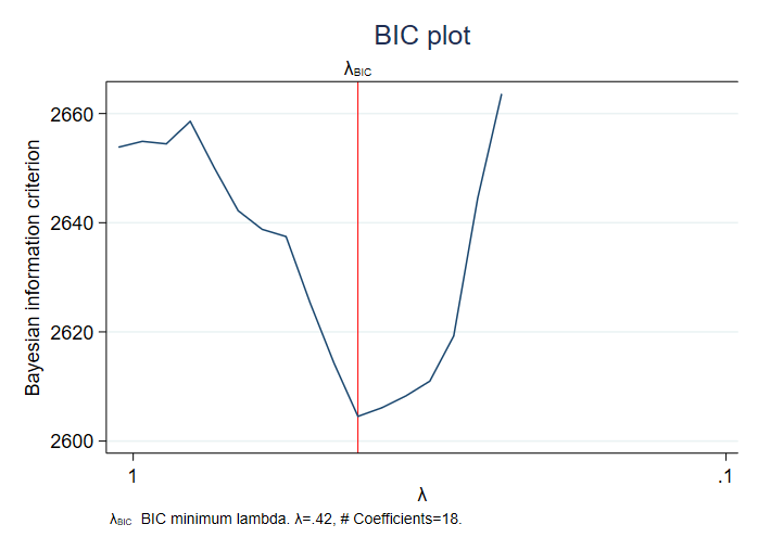
The BIC function decreases quickly before the minimum at λ=0.42.

Using BIC in dsregress for inference

Suppose we are interested in knowing the effect of air pollution (no2_class) on childrens' reaction time (react), controling for covariates. However, we are uncertain about which control variables to include in the model. We can use dsregress to consistently estimate the coefficient on no2_class while using lasso to select control variables.

We specify the selection(bic) option to use bic to select the penalty parameter in each lasso performed by dsregress. We include a set of 32 controls stored in the global macros cc and fc.

. dsregress react no2_class, controls($cc i.($fc)) selection(bic)

Estimating lasso for react using BIC
Estimating lasso for no2_class using BIC

Double-selection linear model         Number of obs               =      1,036
                                      Number of controls          =         32
                                      Number of selected controls =         11
                                      Wald chi2(1)                =      22.18
                                      Prob > chi2                 =     0.0000



            
 
               Robust                                           
       react
 
 Coefficient  std. err.      z    P>|z|     [95% conf. interval]

   no2_class
 
   2.315295   .4916547     4.71   0.000      1.35167    3.278921

. bicplot, for(react)

. bicplot, for(no2_class)