
1 item has been added to your cart.
When analyzing complex survey data, we take into account the characteristics of the survey design—clustering, stratification, sampling weights, and finite-population corrections. We adjust both point estimates and standard errors for the design characteristics when fitting our model, in this case, a structural equation model.
Say we have a sample of employees from a large department store chain who have responded to a series of questions related to job satisfaction. We want to fit a confirmatory factor analysis (CFA) model that measures job satisfaction based on these items. If our data were collected by first sampling stores and then sampling employees within stores, we could adjust the results of our CFA model for this design.
Perhaps we are interested in fitting a multilevel mediation model evaluating whether the impact of one-on-one tutoring influences the relationship between math test scores in third grade and math test scores in fourth grade. We also believe that school-level characteristics might impact test scores and include a school-level random intercept in the model. If the data were collected by first sampling schools and then sampling students within schools, we could adjust the results of our multilevel mediation model for this design.
Throughout Stata, analyzing complex survey data is as simple as using svyset to declare aspects of the survey design and then adding the svy: to the estimation command for the model you want to fit. We can now use svyset and svy: when fitting multilevel structural equation models and structural equation models with binary, count, ordinal, and survival-time outcomes.
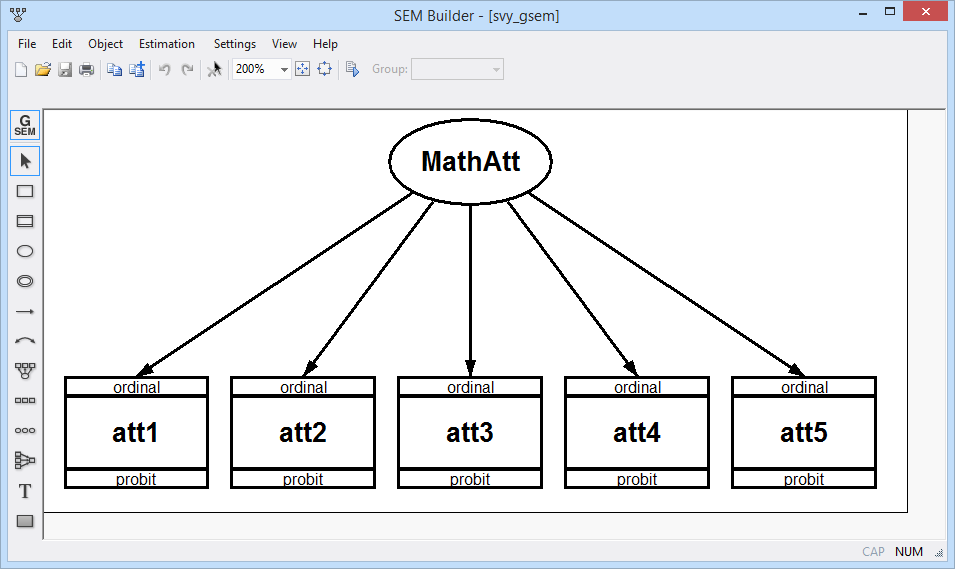
Suppose we are interested in measuring students' attitudes toward math. Our data contain five variables, att1–att5, recording students' responses to various statements about mathematics, such as "skills taught in my math class will help me get a better job" and "I am able to learn new math concepts easily". Responses are coded one through five, with one indicating strong disagreement and five indicating strong agreement with the statement. We want to fit a one-factor CFA model using an ordinal probit model for each response. We name our latent variable MathAtt. If we had random (i.i.d.) data, we could fit the model by typing
. gsem (MathAtt -> att1 att2 att3 att4 att5), oprobit
However, we want to take into account the complex survey design used to collect these data. Schools were sampled first. Then, students were sampled within the selected schools. We have a weight variable, finalwt, that represents the inverse of the probability that a student was included in the sample. We can declare our survey design by typing
. svyset school [pweight=finalwt]
Then, we simply add svy: to gsem:
. svy: gsem (MathAtt -> att1 att2 att3 att4 att5), oprobit

Survey: Generalized structural equation model

Number of strata   =         1                    Number of obs     =        200
Number of PSUs     =        20                    Population size   =      2,852
                                                  Design df         =         19
(output omitted)


 ( 1)  [att1]MathAtt = 1
| Linearized | ||
| Coef. Std. Err. t P>|t| [95% Conf. Interval] | ||
| att1 <- | ||
| MathAtt | 1 (constrained) | |
| att2 <- | ||
| MathAtt | .2771797 .1553982 1.78 0.090 -.0480726 .6024319 | |
| att3 <- | ||
| MathAtt | -1.371444 .4569308 -3.00 0.007 -2.327811 -.4150767 | |
| att4 <- | ||
| MathAtt | -.6330853 .2979832 -2.12 0.047 -1.256771 -.0093992 | |
| att5 <- | ||
| MathAtt | .2898887 .0826312 3.51 0.002 .1169396 .4628377 | |
| att1 | ||
| /cut1 | -.6870853 .1207852 -5.69 0.000 -.9398916 -.4342791 | |
| /cut2 | -.2208128 .1088893 -2.03 0.057 -.4487207 .0070952 | |
| /cut3 | .1666948 .1363675 1.22 0.237 -.1187256 .4521153 | |
| /cut4 | .7558114 .1538749 4.91 0.000 .4337475 1.077875 | |
| att2 | ||
| /cut1 | -.6604855 .1170593 -5.64 0.000 -.9054934 -.4154776 | |
| /cut2 | -.1540785 .0915831 -1.68 0.109 -.3457641 .037607 | |
| /cut3 | .2192101 .1231445 1.78 0.091 -.0385342 .4769544 | |
| /cut4 | .6722401 .1248856 5.38 0.000 .4108516 .9336287 | |
| att3 | ||
| /cut1 | -.6481039 .1283596 -5.05 0.000 -.9167636 -.3794441 | |
| /cut2 | -.0758889 .1233381 -0.62 0.546 -.3340385 .1822606 | |
| /cut3 | .156043 .1375536 1.13 0.271 -.13186 .4439461 | |
| /cut4 | .9826656 .2091878 4.70 0.000 .5448305 1.420501 | |
| att4 | ||
| /cut1 | -.4740356 .1122882 -4.22 0.000 -.7090575 -.2390136 | |
| /cut2 | .0305898 .1162581 0.26 0.795 -.2127411 .2739208 | |
| /cut3 | .4324498 .1159254 3.73 0.001 .1898151 .6750844 | |
| /cut4 | 1.052157 .1762432 5.97 0.000 .6832755 1.421038 | |
| att5 | ||
| /cut1 | -.8521868 .1082836 -7.87 0.000 -1.078827 -.6255467 | |
| /cut2 | -.2671469 .0991305 -2.69 0.014 -.4746295 -.0596644 | |
| /cut3 | .0255667 .0993826 0.26 0.800 -.1824425 .2335779 | |
| /cut4 | .4592799 .0925456 4.96 0.000 .2655797 .65298 | |
| var(MathAtt) | .8373325 .2944519 .4010956 1.748027 | |
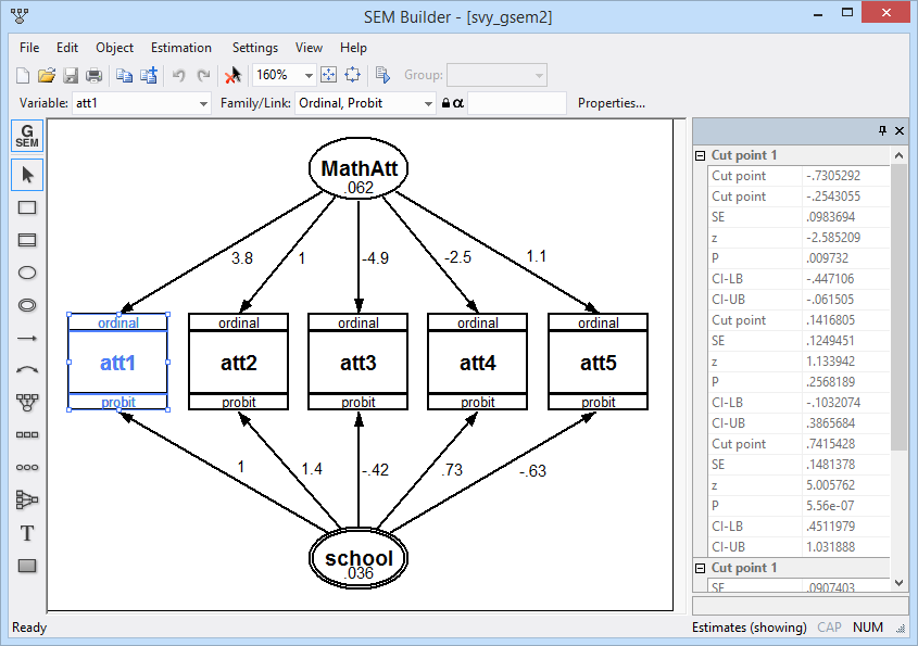
We find the details of our survey design at the top of the output, and the results are adjusted to account for the sampling weights and clusters (schools).
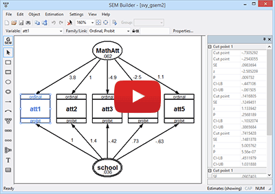
By the way, we could have specified this model and the sample design from Stata's SEM Builder (shown at the top of this page).
gsem also fits multilevel models. For instance, we can add a school-level latent variable to our model above and fit a two-level CFA model.
Ignoring the survey nature of the data, we could fit this model with the following gsem:
. gsem (MathAtt Sch[school] -> att1 att2 att3 att4 att5), oprobit
We have added Sch[school], a latent variable that varies across schools but is constant within school.
As before, we can add svy: to gsem to account for the complex survey design. However, because this is a multilevel model, it is no longer sufficient to provide a single sampling weight. Instead, we need weights for each stage of the design. Here, wt_school is the inverse of the probability that a school is included in the sample, and wt_student is the inverse of the probability that a student is selected, conditional on the student's school being selected.
We can specify weights for both stages of our sampling design using svyset,
. svyset school, weight(wt_school) || _n, weight(wt_student)
and add svy: to gsem:
. svy: gsem (MathAtt Sch[school] -> att1 att2 att3 att4 att5), oprobit

Survey: Generalized structural equation model

Number of strata   =         1                  Number of obs     =        200
Number of PSUs     =        20                  Population size   =      2,852
                                                Design df         =         19
(output omitted)

 ( 1)  [att1]Sch[school] = 1
 ( 2)  [att2]MathAtt = 1
| Linearized | ||
| Coef. Std. Err. t P>|t| [95% Conf. Interval] | ||
| att1 <- | ||
| Sch[school] | 1 (constrained) | |
| MathAtt | 3.750817 2.226429 1.68 0.108 -.9091513 8.410786 | |
| att2 <- | ||
| Sch[school] | 1.432449 1.681672 0.85 0.405 -2.087332 4.955229 | |
| MathAtt | 1 (constrained) | |
| att3 <- | ||
| Sch[school] | -.42361 .9701398 -0.44 0.667 -2.454136 1.606916 | |
| MathAtt | -4.851409 1.890209 -2.57 0.019 -8.807661 -.8951565 | |
| att4 <- | ||
| Sch[school] | .7266975 .340286 2.14 0.046 .0144708 1.438924 | |
| MathAtt | -2.513256 .8880905 -2.83 0.011 -4.372051 -.6544611 | |
| att5 <- | ||
| Sch[school] | -.6266985 .5168374 -1.21 0.240 -1.708452 .4550546 | |
| MathAtt | 1.135442 .9315462 1.22 0.238 -.8143069 3.08519 | |
| att1 | ||
| /cut1 | -.7305292 .0907403 -8.05 0.000 -.9204509 -.5406074 | |
| /cut2 | -.2543055 .0983694 -2.59 0.018 -.4601951 -.0484159 | |
| /cut3 | .1416805 .1249451 1.13 0.271 -.1198326 .4031936 | |
| /cut4 | .7415428 .1481378 5.01 0.000 .4314867 1.051599 | |
| att2 | ||
| /cut1 | -.7283758 .1420862 -5.13 0.000 -1.025766 -.4309859 | |
| /cut2 | -.2056373 .1128682 -1.82 0.084 -.4418732 .0305986 | |
| /cut3 | .177643 .1451251 1.22 0.236 -.1261072 .4813933 | |
| /cut4 | .6475124 .1137837 5.69 0.000 .4093603 .8856645 | |
| att3 | ||
| /cut1 | -.6205503 .1237676 -5.01 0.000 -.8795989 -.3615016 | |
| /cut2 | -.0617385 .1310594 -0.47 0.643 -.336049 .2125719 | |
| /cut3 | .1648772 .1380369 1.19 0.247 -.1240374 .4537918 | |
| /cut4 | .9734501 .1964896 4.95 0.000 .5621925 1.384708 | |
| att4 | ||
| /cut1 | -.5098891 .1165072 -4.38 0.000 -.7537414 -.2660368 | |
| /cut2 | .0085082 .1104815 0.08 0.939 -.2227323 .2397487 | |
| /cut3 | .4231022 .1150956 3.68 0.002 .1822042 .6640001 | |
| /cut4 | 1.061425 .1803608 5.89 0.000 .6839252 1.438924 | |
| att5 | ||
| /cut1 | -.8421634 .1114145 -7.56 0.000 -1.075357 -.6089701 | |
| /cut2 | -.250422 .0987399 -2.54 0.020 -.457087 -.043757 | |
| /cut3 | .0454256 .1016289 0.45 0.660 -.1672861 .2581374 | |
| /cut4 | .4840911 .0949759 5.10 0.000 .2853043 .6828779 | |
| var(Sch[school]) | .0359937 .0334003 .005161 .2510273 | |
| var(MathAtt) | .0616949 .0577655 .0086927 .4378693 | |
As with the previous example, point estimates and standard errors now appropriately account for the complex survey design.
Here is how the model looks when drawn and fit in the SEM Builder.
Although our examples above focus on CFA models, support for complex survey data is available for all models fit by gsem, including one-level and multilevel path models, structural equation models, growth curve models, and more.
Learn more about fitting models with survey data in Stata Structural Equation Modeling Reference Manual.


