Home  /  Stata News  /  Vol 30 No 1 (2015 quarter 1)  /  New in SEM (structural equation modeling)
Stata Release 14: Available now

New in SEM (structural equation modeling)

  • Survival models (parametric)
    • Latent predictors
    • Mediation models and more
    • Unobserved components
    • Multilevel survival models—random intercepts and random coefficients
    • Survival outcomes with other outcomes
    • Right-censoring
    • Left-truncation
    • Exponential, loglogistic, Weibull, lognormal, and gamma survival distributions
  • Generalized models now support survey data
    • Adjusted point estimates, SEs, and tests
    • Observation-level sampling weights
    • Sampling weights at each stage of survey (multilevel models)
    • Clustered sampling
    • Stratified sampling and poststratification
    • Finite population corrections
    • Linearized, bootstrap, jackknife, or BRR standard errors
  • Satorra–Bentler scaled Χ2
    • Adjustment for nonnormal data
    • All relevant goodness-of-fit statistics adjusted
    • Robust standard errors and postestimation tests

What is SEM?

SEM handles one or more latent (unobserved) variables.
(They can be exogenous or endogenous.)

SEM handles one or more observed endogenous variables (and the structural relationships among them).

SEM handles multilevel random effects and random coefficients.

SEMs can be linear or generalized linear, meaning probit, logit, Poisson, and others.

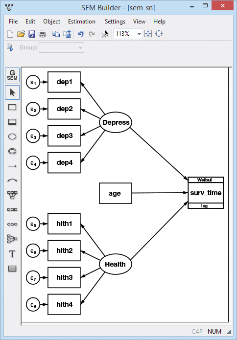
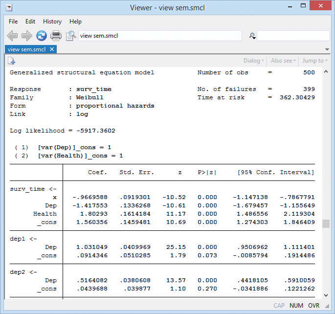
Example 1: Survival model

Let's do a survival model combined with CFA (confirmatory factor analysis). CFAs model the level of a latent trait using observable measurements.

We analyze survival times of nursing home residents. We have censored data; thankfully, not all the residents have died yet.

  • We posit that survival times are determined by age, depression level, and overall health.
  • We have four variables that each measure aspects of depression (our first latent trait).
  • We have four variables that each measure aspects of health (our second latent trait).

We can create our model using Stata's SEM Builder:

SEM Builder

Or we can go directly to typing a command:

. gsem (surv_time <- x Dep Health,
       family(weibull, fail(death)))
       (Depress -> dep1 dep2 dep3 dep4)
       (Health -> hlth1 hlth2 hlth3 hlth4)

Either way, we get the same output:

Generalized structural equation model

SEM produces a lot of output; we've selected just a portion of it.

By the way, another way to think about the observed variables measuring depression and health is that each measures depression (health) with error. Combining the multiple measures allows us to wash away the errors-in-variables bias.

Example 2: Survey data

We want to fit a CFA model for students' attitudes toward math using five ordinal measurements, att1–att5. That's easy enough:

. gsem (MathAtt -> att1 att2 att3 att4 att5), oprobit

However, our data were the result of multiple-stage cluster sampling. Schools were sampled, and then students were sampled from the chosen schools. SEM's new survey features allow us to specify the primary sampling unit and the sampling weight. We just survey set the data:

. svyset school [pweight=finalweight]

If we put svy: in front of the same simple SEM command that we would have typed with random (i.i.d.) data, gsem now produces survey-adjusted results. Just type

.  svy: gsem (MathAtt -> att1 att2 att3 att4 att5), oprobit

running gsem on estimation sample

By the way, we could have specified this entire model, including the survey aspects of the sample, from Stata's SEM Builder.

Upgrade now Order Stata

Read even more about survival models for SEM, Satorra–Bentler adjustments, and survey support for GSEM.