Random-effects panel-data estimators | Order |

It is difficult to say panel data without saying random effects. Panel data are repeated observations on individuals. Random effects are individual-level effects that are unrelated to everything else in the model.
Say we have data on 4,708 employees of a large multinational corporation. We have repeated observations on these employees over the years. On average, we have 6 years of data. For some employees, we have 15 years.
Our data include professional status (1, 2, 3, or 4), age, education, and years of job experience.
We fit the following model:
. xtset idcode year
       panel variable:  idcode (unbalanced)
        time variable:  year, 68 to 88, but with gaps
                delta:  1 unit

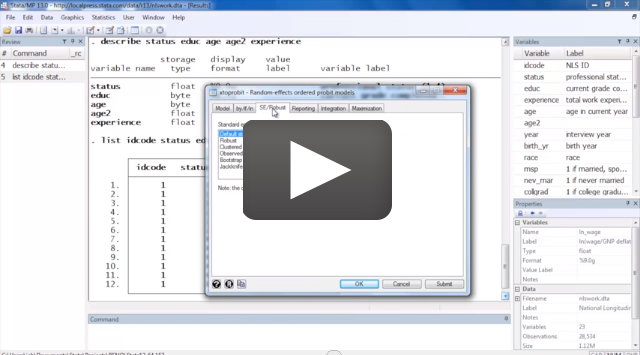
. xtoprobit status educ age age2 experience

Random-effects ordered probit regression        Number of obs      =     28508
Group variable: idcode                          Number of groups   =      4708

Random effects u_i ~ Gaussian                   Obs per group: min =         1
                                                               avg =       6.1
                                                               max =        15

Integration method: mvaghermite                 Integration points =        12

                                                Wald chi2(4)       =   5676.07
Log likelihood  = -26032.326                    Prob > chi2        =    0.0000
| status | Coef. Std. Err. z P>|z| [95% Conf. Interval] | |
| educ | .333993 .0091215 36.62 0.000 .3161152 .3518707 | |
| age | .2129696 .0123513 17.24 0.000 .1887616 .2371777 | |
| age2 | -.004221 .0002029 -20.80 0.000 -.0046188 -.0038232 | |
| experience | .1918314 .004661 41.16 0.000 .1826959 .2009669 | |
| /cut1 | 7.625209 .2156879 35.35 0.000 7.202468 8.047949 | |
| /cut2 | 8.498753 .217015 39.16 0.000 8.073411 8.924094 | |
| /cut3 | 10.07729 .219697 45.87 0.000 9.646696 10.50789 | |
| /sigma2_u | 1.498732 .0506867 1.402609 1.601443 | |
We find that the probability of the highest status level increases with education and experience. We also find that individuals have a large permanent component (/sigma2_u, the variance of the random effect, is both large and significant).
Learn more about random effects ordered probit and logit in the Stata manuals at
See New in Stata 19 to learn about what was added in Stata 19.