1 item has been added to your cart.

Highlights

• Solve for
• Power
• Sample size
• Minimum detectable effect
• Effect size
• Comparisons of
• Means (t tests)
• Proportions
• Variances
• Correlations
• ANOVA models
  • One-way
  • Two-way
  • Repeated-measures
• Designs
• Matched case–control studies
• Cohort studies
• Cross-sectional studies
• Tables and graphs
• Automated
• Custom
• Add your own methods
• Automated tables
• Automated graphs

Show me

Say we are planning an experiment to determine whether students who prepare for the SAT exam obtain higher math scores by (1) taking classes rather than (2) studying independently. The national average math score is 520 with a standard deviation of 135. We want to see the power obtained for sample sizes of 100 through 500 when scores increase by 20, 40, 60, and 80 points or, equivalently, when average scores increase to 540, 560, 580, and 600.

We type

. power twomeans 520 (540 560 580 600), n(100 200 300 400 500) sd(135) graph

We assumed above that those studying independently would obtain the national average of 520 and that the standard deviations would be 135 for both groups. We could relax either assumption using the power command.

We might be more interested in the sample size necessary to detect the increased scores at power levels of 0.8 and 0.9. In that case, we type

. power twomeans 520 (540 560 580 600), power(0.8 0.9) sd(135) graph

We can even estimate the detectable increased scores over the range of sample sizes and powers:

. power twomeans 520, power(0.8 0.9) n(100 200 300 400 500) sd(135) graph

If we prefer to see the detectable limits as effect sizes (difference between the experimental group mean and the control group mean) rather than experimental-group test scores, we add option y(delta) to the command:

. power twomeans 520, power(0.8 0.9) n(100 200 300 400 500) sd(135) graph(y(delta))

In this graph, the effect size is calculated as (experimental group mean - 520).

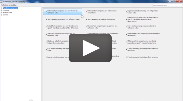
In our example, we dealt with a comparison of means across two independent samples. power can produce comparisons of means, proportions, variances, and correlations for one and two samples and comparisons of means and proportions for paired samples.

Show me more

See the all-new 262-page Power and Sample Size Manual, especially the introduction.

And see the worked examples:

One-sample comparison of means
One-sample comparison of proportions
One-sample comparison of variances
One-sample comparison of correlations
Comparison of two independent means
Comparison of two independent proportions
Comparison of two independent variances
Comparison of two independent correlations
Comparison of two paired means
Comparison of two paired proportions
One-way ANOVA
Two-way ANOVA
Repeated measures ANOVA

Back to highlights

See New in Stata 18 to learn about what was added in Stata 18.