1 item has been added to your cart.

Highlights

• More flexible parameterization than with polynomials
• Prefix command for use with any estimation command

Show me

Fractional polynomials are an alternative to regular polynomials that provide flexible parameterization for continuous variables.

For example, say we have an outcome y, a regressor x, and our research interest is in the effect of x on y. We know that y is also affected by age. One solution to this problem would be to fit a linear regression of the form

           yi = b0 + b1*xi + b2*agei + b3*agei2 + ui

An alternative would be to control for age using fractional polynomials:

           yi = b0 + b1*xi + b2*agei(p1) + b3*agei(p2) + ui

The parentheses are significant. Fractional powers are different from regular powers. For instance, age⁽⁰⁾ is ln(age). You can see the full definition, but one example will demonstrate the power of fractional polynomials.

To fit the fractional polynomial model, we type

. fp <age>: regress y x <age>
(fitting 44 models)
(....10%....20%....30%....40%....50%....60%....70%....80%....90%....100%)

Fractional polynomial comparisons:



         age 
 
   df    Deviance  Res. s.d.   Dev. dif.   P(*)   Powers

 
 
 

     omitted 
 
    0    -83.145      0.237    625.517    0.000               

      linear 
 
    1   -179.287      0.232    529.376    0.000   1           

       m = 1 
 
    2   -295.392      0.225    413.270    0.000   3           

       m = 2 
 
    4   -708.663      0.203      0.000       --   -.5 -.5     



(*) P = sig. level of model with m = 2 based on F with 1994
    denominator dof.


      Source 
 
       SS       df       MS   
           Number of obs =    2000

 
 
 
           F(  3,  1996) =  347.37

       Model 
 
  42.8971855     3  14.2990618
           Prob > F      =  0.0000

    Residual 
 
  82.1620986  1996  .041163376
           R-squared     =  0.3430

 
 
 
           Adj R-squared =  0.3420

       Total 
 
  125.059284  1999  .062560923
           Root MSE      =  .20289




           y 
 
      Coef.   Std. Err.      t    P>|t|     [95% Conf. Interval]

 
 
 

           x 
 
   .7954347   .0466225    17.06   0.000     .7040008    .8868686

       age_1 
 
   11.04709   .4085977    27.04   0.000     10.24577    11.84841

       age_2 
 
   13.17616   .4991682    26.40   0.000     12.19722    14.15511

       _cons 
 
  -8.059393   .5469551   -14.74   0.000    -9.132056    -6.98673

We find that b₁, the effect of x on y, is 0.80, but before we take that result seriously, we must ask ourselves whether we have adequately controlled for age.

. fp plot, residuals(none)

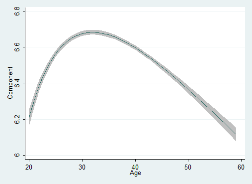
Notice the shape of the y versus age curve. We could not have obtained that shape using a standard quadratic. Fractional polynomials provide a wide range of shapes that include all the shapes provided by ordinary polynomials and more. The fractional polynomial parameterization did not predetermine that the shape we obtained was skewed right. Fractional polynomials can just as easily produce skewed left shapes.

We still need to do more to convince ourselves that the curve above is adequate, but we will not do so here.

Show me more

See the fractional polynomial manual entry.

Back to highlights

See New in Stata 18 to learn about what was added in Stata 18.