1 item has been added to your cart.

See the video

Highlights

Time-series and panel datasets Multiple estimation results OLS, VARs, VECs, ARIMAs, ARCHs, 3SLS, and more Estimated with Stata or obtained from outside sources One equation or thousands Identities Add factors and other adjustments Dynamic or static (one-step-ahead) forecasts Solve simultaneous systems Confidence intervals via stochastic simulation Compare forecasts of alternative scenarios

Show me

We will forecast a simple seven-equation model produced by one estimation command, but we could forecast a model with thousands of equations obtained from thousands of estimation commands.

We fit a classic model (Klein 1950) of the US economy to pre-World War II data using 3SLS:

. reg3 (c p L.p w) (i p L.p L.k) (wp y L.y yr), endog(w p y) exog(t wg g)
  (output omitted)

. estimates store klein 

Now we tell forecast about our estimation results and the model's identities:

Even better, we could have entered the above into forecast's Control Panel:

The result is

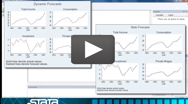
That may look boring, but forecast has saved our forecast. We could graph the results:

Notice how easy this all was. We used reg3 to fit stochastic equations for three variables, and we stored our estimation results. We then created a forecast model named kleinmodel and added those results. This model has only one set of estimation results, but we could have added more. We then defined a few identities that describe other variables in our model. The first one is familiar to introductory economics students: the nation's income is the sum of consumption, investment, and government spending (ignoring foreign trade). This period's capital stock is just last year's capital stock plus net investment, where investment was one of the equations in our 3SLS model. We told forecast about our exogenous variables; then we told it to solve our model.

By default, forecast produces dynamic forecasts, but we could have asked for static ones instead. Moreover, we could have asked forecast to estimate the amount of error surrounding our forecast by accounting for variability stemming from parameter uncertainty as well as additive error terms.

forecast also lets you specify alternative paths for some variables and obtain forecasts for the other variables in the model conditional on those paths. That way, you can perform policy simulations and develop forecasts assuming a range of different scenarios.

Show me more

Learn much more about forecasting in Stata by reading the manual entry.

Back to highlights

See New in Stata 18 to learn about what was added in Stata 18.