Unobserved components model (UCM)

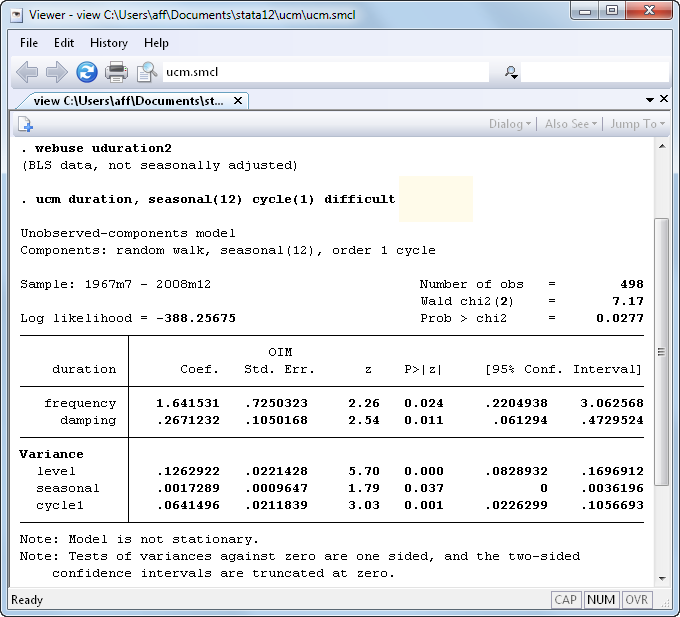
Stata’s new ucm command estimates the parameters of an unobserved components model (UCM). UCM decomposes a time series into trend, seasonal, cyclical, and idiosyncratic components and allows for exogenous variables. UCM is an alternative to ARIMA models and provides a flexible and formal approach to smoothing and decomposition problems.

Here we fit monthly data on the median duration of unemployment spells in the United States to a stochastic cycle model with a stochastic seasonal component because the data have not been seasonally adjusted.

Important components are components with a large spectral density, and, thus, the estimated damping parameter specifies how tightly the important components are distributed around the estimated central frequency. We calculate and plot the spectral density implied by these parameter estimates below.

. psdensity omega density 

. twoway line omega density

Moving on to prediction, we predict the trend and the seasonal components:

. predict strend, trend

. predict season, seasonal

Below we graph the trend component in the top panel and the seasonal component in the bottom panel.

We can also forecast the median unemployment duration and graph the results.

. tsappend, add(12)

. predict duration_f, dynamic(tm(2009m1)) rmse(rmse)

For a complete list of what’s new in time-series analysis, click here.

Back to highlights

See New in Stata 17 to learn about what was added in Stata 17.