1 item has been added to your cart.

Time-series filters

The new tsfilter command separates a time series into trend and cyclical components. The trend component may contain a deterministic or a stochastic trend. The stationary cyclical component is driven by stochastic cycles at the specified periods.

Many time series contain trends and are thus nonstationary. Fitting nonstationary time series to statistical models can be difficult. Some researchers use filters to remove the trends and analyze the stationary components that the filters leave behind.

tsfilter implements the Baxter–King, Butterworth, Christiano–Fitzgerald, and Hodrick–Prescott filters commonly used for this purpose.

For example, we have quarterly data on GDP from 1952 through 2010.

. webuse gdp2
(Federal Reserve Economic Data, St. Louis Fed)

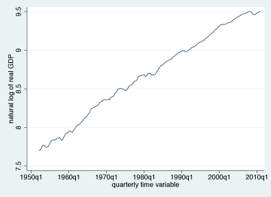
The data are strongly trended. Here is a graph of gdp_ln, the log of GDP over time, variable :

We will use a Baxter–King band-pass filter for this series. Band-pass filters remove components below the minimum frequency or above the maximum frequency. Below we specify we want to remove frequencies with periods shorter than 6 months or longer than 32 months.

. tsfilter bk gdp_bk = gdp_ln, minperiod(6) maxperiod(32)

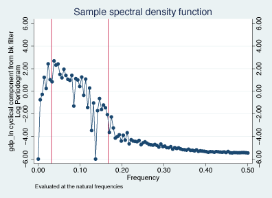
We have now created new variable gdp_bk containing the filtered series. To evaluate how the filter performed, we use Stata’s pergram command to compute and plot the periodogram of the filtered series. We put vertical lines at the minimum and maximum frequencies (1/32 and 1/6). If the filter did exactly want we want, the periodogram would be a horizontal line below the minimum and above the maximum frequencies.

While the Baxter–King filter performed adequately, perhaps the Butterworth filter could do better. The Butterworth filter is a high-pass filter, meaning that it only removes the low-frequency components. High-pass filters can be used to make band-pass filters, but here we will just look at the high-pass results. The Butterworth filter has a tuning parameter called the order of the filter. We set the order of the filter to 8 in the application below.

. tsfilter bw gdp_bw = gdp_ln, order(8) maxperiod(32)

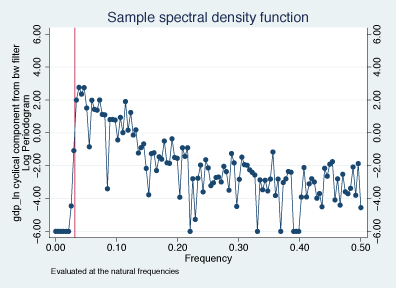
The resulting periodogram for this filtered series is

The periodogram indicates that the Butterworth filter did a better job of removing the low-frequency components than the Baxter–King filter did.

We could continue with this story. We would filter the series using the Christiano–Fitzgerald band-pass filter and the Hodrick–Prescott high-pass filter and compare the results. The Christiano–Fitzgerald filter would produce results rivaling the Butterworth filter. The Hodrick–Prescott filter would not perform as well with these data.

For a complete list of what’s new in time-series analysis, click here.

Back to highlights

See New in Stata 18 to learn about what was added in Stata 18.