1 item has been added to your cart.

Structural equation modeling (SEM)

If you don’t know what SEM is, go here.

View the complete list of SEM capabilities

SEM stands for structural equation modeling. SEM is a notation for specifying structural equations, a way of thinking about them, and methods for estimating their parameters.

SEM encompasses a broad array of models from linear regression to measurement models to simultaneous equations, including along the way confirmatory factor analysis (CFA), correlated uniqueness models, latent growth models, and multiple indicators and multiple causes (MIMIC).

Stata’s new sem command fits SEMs.

Features

• Use GUI or command language to specify model.
• Standardized and unstandardized results.
• Direct and indirect effects.
• Goodness-of-fit statistics.
• Tests for omitted paths and tests of model simplification including modification indices, score tests, and Wald tests.
• Predicted values and factor scores.
• Linear and nonlinear (1) tests of estimated parameters and (2) combinations of estimated parameters with CIs.
• Estimation across groups is as easy as adding group(sex) to the command. Test for group invariance. Easily add or relax constraints across groups.
• SEMs may be fitted using raw or summary statistics data.
• Maximum likelihood (ML) and asymptotic distribution free (ADF) estimation. ADF is also known as generalized method of moments (GMM). Missing at random (MAR) data supported via FIML.
• Robust estimate of standard errors and standard errors for clustered samples available.
• Support for survey data including sampling weights, stratification and poststratification, and clustered sampling at one or more levels.

GUI or commands, it’s your choice

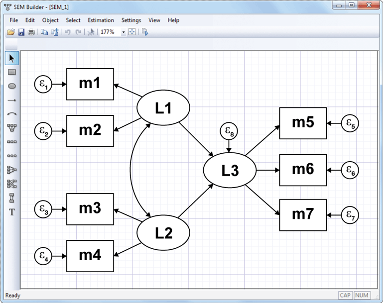
Enter your model graphically,

or use the command syntax

. sem (L1 -> m1 m2)
      (L2 -> m3 m4)
      (L3 <- L1 L2)
      (L3 -> m5 m6 m7)

It’s the same model either way.

Stata’s GUI uses standard path notation.

In command syntax, you type the path diagram. Capitalized names are latent variables. Lowercased names are observed variables. You can type arrows in either direction. The above model could be equally well typed as

. sem (m1 m2 <- L1)
      (L2 -> m3 m4)
      (L3 <- L1 L2)
      (L3 -> m5 m6 m7)

and order does not matter, and neither does spacing:

. sem (m1 m2 <- L1) (L2 -> m3 m4) (L3 -> m5 m6 m7) (L3 <- L1 L2)

You can specify paths individually,

. sem (m1 <- L1) (m2 <- L1) (L2 -> m3) (L2 -> m4)  (L3 -> m5) (L3 -> m6) (L3 -> m7) (L3 <- L1) (L3 <- L2)

or combined,

. sem (m1 m2 <- L1) (L2 -> m3 m4) (L3 -> m5 m6 m7) (L3 <- L1 L2)

Show me

Let’s fit a structural model with a measurement component using data from Wheaton, Muthén, Alwin, and Summers (1977):

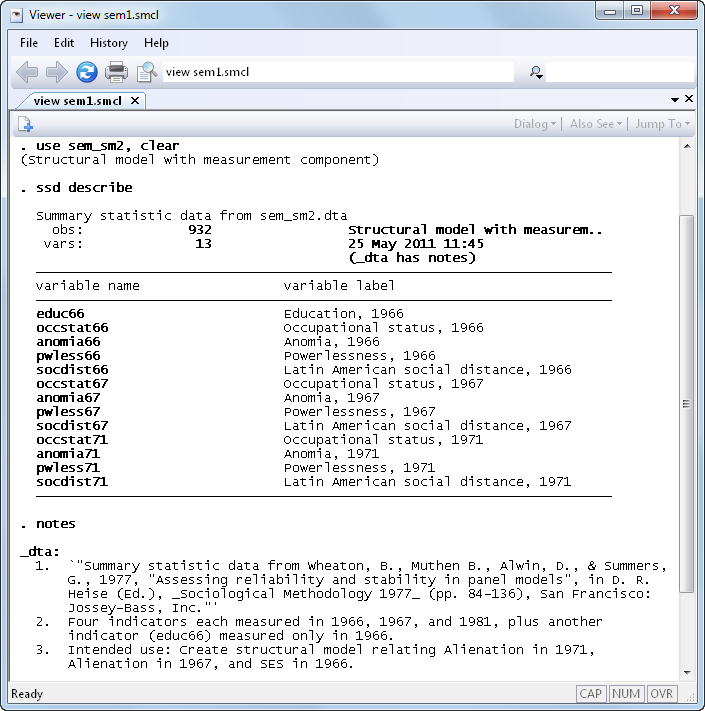
Below we will demonstrate

• Fitting the model
• Modification indices
• Refitting the model

Show me, fitting the model

Simplified versions of the model fit by the authors of the referenced paper appear in many SEM software manuals. One simplified model is

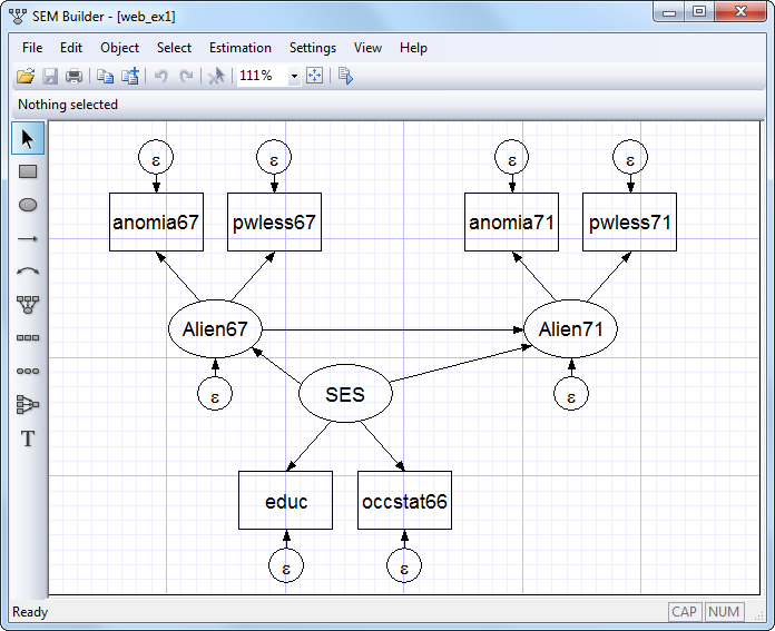
You can also readily fit this model using the following command:

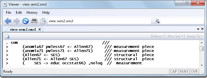
And the results are

Notes:

1. Measurement component: In both 1967 and 1971 anomia and powerlessness are used to measure endogenous latent variables representing Alienation for the same two years. Education and occupational status are used to measure the exogenous latent variable SES.
2. Structural component: SES->Alien67 and SES->Alien71, and Alien67->Alien71.
3. The model vs. saturated chi-squared test indicates the model is a poor fit.

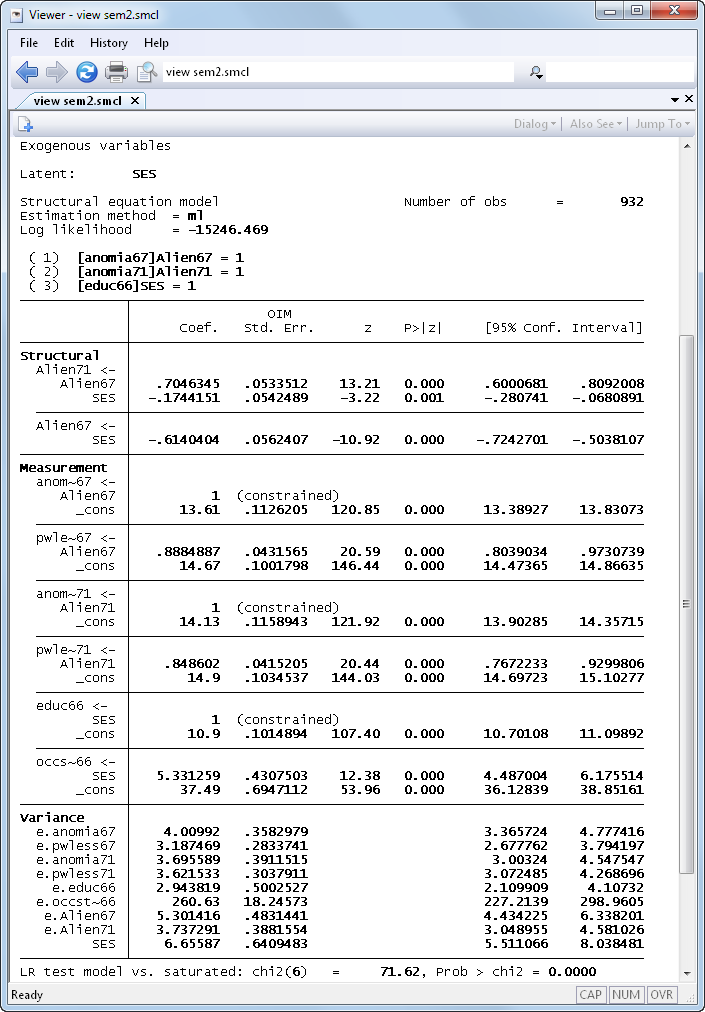
Show me, modification indices

That the model is a poor fit leads us to looking at the modification indices:

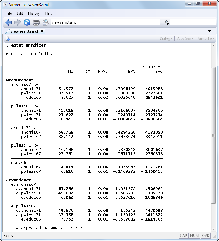
Notes:

1. There are lots of statistically significant paths we could add to the model.
2. Some of those statistically significant paths also make theoretical sense.
3. Two in particular that make sense are the covariances between e.anomia67 and e.anomia71, and between e.pwless67 and e.pwless71.

Show me, refitting the model

Let’s refit the model and include those two previously excluded covariances:

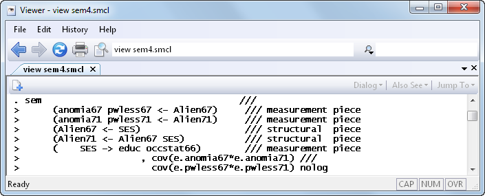
And the results are

Notes:

1. We find the covariance between e.anomia67 and e.anomia71 to be significant(Z=5.14).
2. We find the covariance between e.pwless67 and e.pwless71 to be insignificant at the 5% level (Z=1.29).

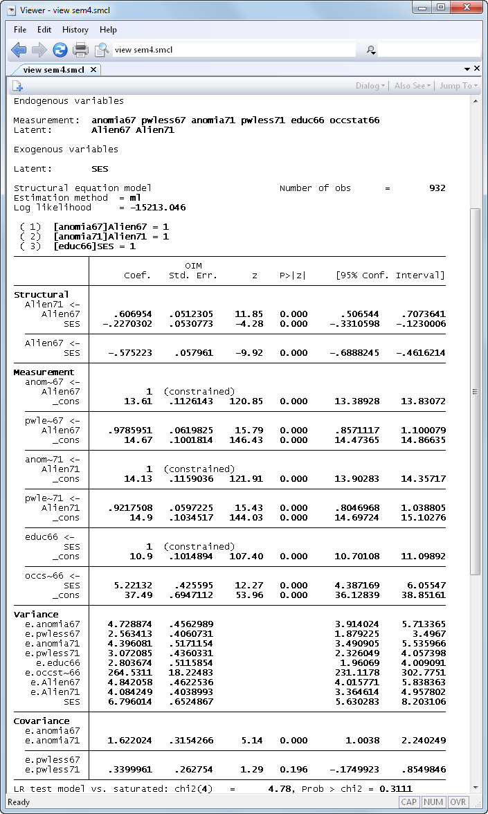
Back to highlights

See New in Stata 18 to learn about what was added in Stata 18.