
1 item has been added to your cart.
Parametric spectral density estimation was introduced in Stata 12.
Order |
A stationary process can be decomposed into random components that occur at different frequencies. The spectral density of a stationary process describes the relative importance of these random components.
Stata’s new psdensity command estimates the spectral density of a stationary process using the parameters of a previously estimated parametric model.
Consider the changes in the number of manufacturing employees in the United States:
. webuse manemp2
(FRED data: Number of manufacturing employees in U.S.)
The horizontal line corresponds to the mean. There appear to be more runs above the mean, and more runs below the mean, than we would expect from a series without autocorrelation. These runs suggest positive autocorrelation.
Fitting these data to a first-order autoregressive process confirms our suspicions:
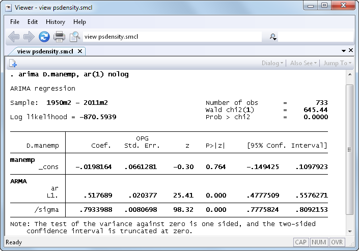
The statistically significant estimate of 0.518 for the autoregressive coefficient indicates that there is an important amount of positive autocorrelation in this series.
Next we can use psdensity to estimate the spectral density of the process implied by the estimated parameters.
. psdensity density omega

. twoway line density omega
The above graph is typical of a spectral density of an AR(1) process with a positive coefficient. The curve is highest at frequency 0, and it tapers off toward zero or a positive asymptote. This estimated spectral density tells us that the low-frequency random components are the most important random components of an AR(1) process with a positive autoregressive coefficient.
For a complete list of what’s new in time-series analysis, click here.
See New in Stata 19 to learn about what was added in Stata 19.


