

In the spotlight: Bayesian vector autoregressive models
Vector autoregressive models (VARs) have been widely used in macroeconomics to summarize data interdependencies, test generic theories, and conduct policy analyses (Canova 2007). The application of Bayesian VAR models, however, has been more limited, mostly because of the difficulties in specifying and fitting such models. The Bayesian approach to modeling multiple time series provides some distinct advantages to the classical approach, some of which I try to illustrate here in this article. Specifically, I apply Bayesian vector autoregression to model the relationships between gross domestic product (GDP), labor productivity, and CO2 emissions, and I show that the Bayesian approach in Stata is no more complicated than the classical approach.
You can read more about classical VAR models in my colleague David Schenck's blog post Vector autoregressions in Stata.
Bayesian VAR models are available in Stata 17 through the new bayes: var command as part of the Bayesian economics suite; see [BAYES] bayes: var for more details.
CO2 emissions data
In the last couple of decades, the effect of economic activity on the environment has been a subject of ever-increasing research (Grossman and Krueger 1993). Of particular interest has been the link between economic output and CO2 emissions (Grossman and Krueger 1995).
The dataset I use, greensolow, is from chapter 5 of Environmental Econometrics Using Stata (Baum and Hurn 2021). Also there, you can find examples of standard VAR analysis.
The dataset contains quarterly observations of per capita CO2 emissions (co2) and various economic factors such as real per capita GDP (gdp), labor productivity (lp), and others. datevec is the time variable. Below is the description of the variables in the dataset.
. use greensolow

. describe

Contains data from greensolow.dta
 Observations:           282
    Variables:             8                  28 Aug 2018 11:13
                                              (_dta has notes)
| Variable Storage Display Value |
| name type format label Variable label |
| datevec float %tq co2 double %9.0g * quarterly per capita co2 emissions gdp float %9.0g real per capita gdp lp float %9.0g labour productivity tfp float %9.0g quarterly utilization adjusted total factor productivity p float %9.0g relative price of investment rc float %9.0g real personal consumption expenditure spread float %9.0g credit spread on corporate bond yields * indicated variables have notes |
We rescale the gdp and co2 variables to make them comparable in range and facilitate the interpretation of the regression results later.
. replace gdp = gdp/1000
(274 real changes made)

. replace co2 = co2*1000
(173 real changes made)

. summarize gdp lp co2
| Variable | Obs Mean Std. dev. Min Max | |
| gdp | 274 7.890994 4.510167 1.989535 16.57506 | |
| lp | 274 91.17146 31.7574 40.46978 148.8792 | |
| co2 | 173 6.609467 .6417095 4.932328 8.125009 |
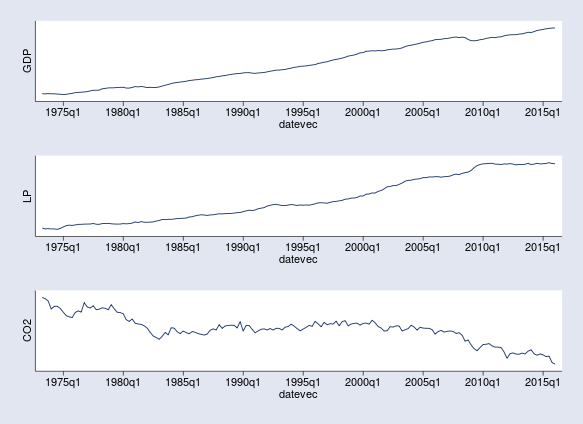
Let's first have a quick look at the observed three time series of interest: gdp, lp, and co2. There are no data available for CO2 emissions before the second quarter of 1973. Hence, we restrict the range of the tsline commands.
. tsline gdp if tin(1973q2,2016q1), ytitle("GDP") ylabel(none) nodraw name(tsline1)

. tsline lp if tin(1973q2,2016q1), ytitle("LP") ylabel(none) nodraw name(tsline2)

. tsline co2 if tin(1973q2,2016q1), ytitle("CO2") ylabel(none) nodraw name(tsline3)

. graph combine tsline1 tsline2 tsline3, rows(3)
It is apparent that the time series are not stationary: gdp and lp have been increasing in time trends, while co2 is distinctively nonlinear. From about 1983 to 2008, per capita CO2 emissions are relatively constant, but there are decreasing trends before 1983 and after 2008, perhaps because of changes in labor productivity. The increasing trends of gdp and lp are also disturbed for short periods around the 2008 recession.
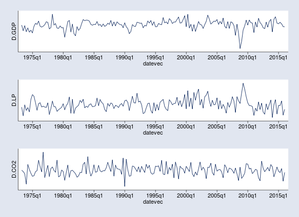
Because VAR models are not directly applicable to nonstationary time series, we consider the first differences D.gdp, D.lp, and D.co2. The first differences are interpreted as growth rates of real GDP, labor productivity, and CO2 emissions. Their time-series graphs show no apparent trends.
. tsline D.gdp if tin(1973q2,2016q1), ytitle("D.GDP") ylabel(none) nodraw name(tsline1)

. tsline D.lp if tin(1973q2,2016q1), ytitle("D.LP") ylabel(none) nodraw name(tsline2)

. tsline D.co2 if tin(1973q2,2016q1), ytitle("D.CO2") ylabel(none) nodraw name(tsline3)

. graph combine tsline1 tsline2 tsline3, rows(3)
Lag order selection
At this point, we are ready to apply a VAR model to D.gdp, D.lp, and D.co2, which, in the context of VAR, we call endogenous variables. A VAR model is nothing but a linear regression of the endogenous variables on their own lags. To specify a VAR model, we first need to choose its lag order. In classical settings, one may use the Stata command varsoc, which provides different information criteria for selecting the order. However, having different criteria complicates the choice because the most popular criteria, AIC and BIC, do not often agree.
In Bayesian settings, we compare models based on their posterior probabilities—we fit models with 1, 2, etc., up to a maximum lag order and compare them using, for example, the bayestest model command in Stata. Below, I consider models with up to four lags and compare them. All model specifications include the Bayes options mcmcsize(1000), for reducing the MCMC sample size; rseed(), for reproducibility; and saving(), for saving MCMC samples.
. quietly bayes, mcmcsize(1000) rseed(17) saving(bsim, replace): var D.gdp D.lp D.co2, lags(1/1)

. estimates store bvar1

. quietly bayes, mcmcsize(1000) rseed(17) saving(bsim, replace): var D.gdp D.lp D.co2, lags(1/2)

. estimates store bvar2

. quietly bayes, mcmcsize(1000) rseed(17) saving(bsim, replace): var D.gdp D.lp D.co2, lags(1/3)

. estimates store bvar3

. quietly bayes, mcmcsize(1000) rseed(17) saving(bsim, replace): var D.gdp D.lp D.co2, lags(1/4)

. estimates store bvar4

. bayestest model bvar1 bvar2 bvar3 bvar4

Bayesian model tests
| log(ML) P(M) P(M|y) | ||
| bvar1 | 102.9553 0.2500 0.9709 | |
| bvar2 | 99.4340 0.2500 0.0287 | |
| bvar3 | 94.9101 0.2500 0.0003 | |
| bvar4 | 93.4377 0.2500 0.0001 | |
The first column in the output table of bayestest model reports the log-marginal likelihoods; the second reports the prior model probabilities, which are all equal to 0.25 by default; and the third column reports the posterior model probabilities. The simplest model with one lag has a probability of 0.97, and it is overwhelmingly the best one.
Fitting the Bayes VAR model
After deciding that a VAR model of order 1 is appropriate for our data, we are ready to specify and fit the model. Recall that a Bayesian model must also include priors for all model parameters. In the case of VAR, we have regression coefficients grouped by equations (one for each endogenous variable) and the variance–covariance matrix of the error terms. The bayes: var command provides a default prior model, the so-called conjugate Minnesota prior, and this is the one we stick with. Because Bayesian estimation is essentially a sampling from the posterior distribution of the model, we add the rseed() option for reproducibility and reduce the MCMC sample size to 1,000, deeming it to be sufficient.
. bayes, mcmcsize(1000) rseed(17): var D.gdp D.lp D.co2, lags(1)

Burn-in ...
Simulation ...

Model summary
| Likelihood: D_gdp D_lp D_co2 ~ mvnormal(3,xb_D_gdp,xb_D_lp,xb_D_co2,{Sigma,m}) Priors: {D_gdp:LD.gdp LD.lp LD.co2 _cons} (1) {D_lp:LD.gdp LD.lp LD.co2 _cons} (2) {D_co2:LD.gdp LD.lp LD.co2 _cons} ~ varconjugate(3,1,1,_b0,{Sigma,m},_Phi0) (3) {Sigma,m} ~ iwishart(3,5,_Sigma0) | ||
| (1) Parameters are elements of the linear form xb_D_gdp. (2) Parameters are elements of the linear form xb_D_lp. (3) Parameters are elements of the linear form xb_D_co2. Bayesian vector autoregression MCMC iterations = 3,500 Gibbs sampling Burn-in = 2,500 MCMC sample size = 1,000 Sample: 1973q3 thru 2016q1 Number of obs = 171 Acceptance rate = 1 Efficiency: min = .8147 avg = .9769 Log marginal-likelihood = 102.95529 max = 1 | ||
| Equal-tailed | ||
| Mean Std. dev. MCSE Median [95% cred. interval] | ||
| D_gdp | ||
| gdp | ||
| LD. | .5796619 .0661197 .002091 .5771234 .4488638 .7079532 | |
| lp | ||
| LD. | -.0174199 .0066842 .000211 -.0177438 -.0295753 -.0041474 | |
| co2 | ||
| LD. | .0357662 .0308744 .000976 .0363394 -.0279287 .095661 | |
| _cons | .0346589 .007285 .000242 .0346453 .0210438 .0484967 | |
| D_lp | ||
| gdp | ||
| LD. | -3.006862 .6266633 .019817 -3.004131 -4.301595 -1.759183 | |
| lp | ||
| LD. | .5432933 .0647291 .002012 .5407274 .4190424 .6696202 | |
| co2 | ||
| LD. | -.0751836 .2995545 .009473 -.0688522 -.6757699 .4919293 | |
| _cons | .3764 .0680885 .002153 .376942 .2442487 .5111251 | |
| D_co2 | ||
| gdp | ||
| LD. | .3252994 .149951 .004396 .3162642 .0197296 .6101307 | |
| lp | ||
| LD. | -.0006642 .0163091 .000517 -.0003933 -.033088 .0289234 | |
| co2 | ||
| LD. | .2342499 .0752377 .002379 .2361941 .0854152 .3770827 | |
| _cons | -.0350984 .0168797 .000572 -.0348312 -.070182 -.0021437 | |
| Sigma_1_1 | .0050236 .0005201 .000014 .005003 .00405 .0060574 | |
| Sigma_2_1 | .0293233 .0041989 .000127 .0290843 .0221124 .038277 | |
| Sigma_3_1 | -.0003943 .0009121 .000027 -.0003756 -.0023657 .001382 | |
| Sigma_2_2 | .4503552 .048543 .001535 .4466805 .3663917 .5593156 | |
| Sigma_3_2 | .0018873 .0085198 .000269 .0017915 -.0143019 .0189473 | |
| Sigma_3_3 | .0272382 .002926 .000103 .0270488 .0220155 .0334743 | |
The bayes: var command uses efficient Gibbs sampling for simulation and rarely has MCMC convergence problems. In this particular run, we have a very high sampling efficiency of 0.98. The MCMC sample of size 1,000 is thus equivalent to about 980 independent draws from the posterior, which provides enough estimation precision.
The output of bayes: var is fairly long because of the large number of regression coefficients: three equations with four coefficients each. Also included is the three-by-three covariance matrix Sigma. In practice, a VAR model is interpreted not through its regression coefficients but by using various impulse–response functions. However, there is one more step that is needed before continuing with the interpretation of results.
Checking model stability
Some postestimation VAR routines such as impulse–response functions are only meaningful for stable VAR models; see [BAYES] bayesvarstable for a precise definition and more details. To check the stability of a Bayesian VAR model, we use the bayesvarstable command. As usual, the simulation results of bayes: var need to be saved first.
. bayes, saving(bvarsim1, replace)
note: file bvarsim1.dta not found; file saved.

. bayesvarstable

Eigenvalue stability condition                    Companion matrix size =    3
                                                  MCMC sample size      = 1000
| Eigenvalue | Equal-tailed | |
| modulus | Mean Std. dev. MCSE Median [95% cred. interval] | |
| 1 | .8019066 .0520921 .001647 .8022324 .700483 .8966506 | |
| 2 | .368717 .083123 .002629 .3626458 .2194205 .5469187 | |
| 3 | .1898191 .0779832 .002466 .1896387 .0343819 .3393437 | |
The bayesvarstable command estimates the moduli of the eigenvalues of the companion matrix of the VAR model, which in this case is 3. Similarly to the frequentist varstable command, bayesvarstable performs unit circle tests but accounting for the fact that, in a Bayesian context, these moduli are random numbers.
The first column in the output table shows the posterior mean estimates for the eigenvalue moduli in decreasing order: 0.80, 0.37, and 0.19. Simply comparing them with 1 is not sufficient for testing stability, though. The most informative output of the command is the posterior probability of unit circle inclusion reported right below the eigenvalue estimation table. It is essentially 1 in our case, assuring the stability of the model. If the inclusion probability is significantly lower than 1, we should suspect instability. The degree of instability thus may vary. Luckily, we don't have an issue here.
Impulse–response functions
Impulse–response functions (IRFs) provide the main toolbox for exploring a VAR model. They consider a shock to one variable (the impulse) and how this shock affects an endogenous variable (the response). The bayesirf create command computes a set of IRFs for each impulse–response pair and saves them in an irf dataset. Please see [BAYES] bayesirf for more details.
Below, we compute IRFs with a length of 20 steps, equivalent to a 5-year period, and save them as a birf1 result in a birf.irf dataset.
. bayesirf create birf1, set(birf) step(20) mcmcsaving(birf1mcmc)
(file birf.irf created)
(file birf.irf now active)
file birf1mcmc.dta saved.
(file birf.irf updated)
Note that birf1 contains Bayesian results such as posterior means, standard deviations, and credible intervals. In addition, I use the mcmcsaving() option to save the MCMC draws for the IRFs in an external dataset. This will allow me to request various posterior summaries for the IRFs afterward, such as different credible-interval levels.
Let's first see the effects of shocks to D.gdp and D.lp on D.co2 in terms of regular IRFs, irf. We use bayesirf cgraph to combine the two IRFs.
. bayesirf cgraph (birf1 D.gdp D.co2 irf) (birf1 D.lp D.co2 irf)
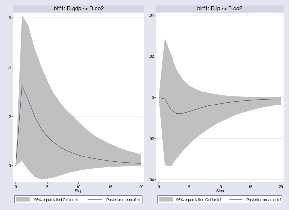
A shock to D.gdp has a positive response on D.co2, but a shock to D.lp has a negative one. Although the results apply to the first differences (growth rates) of our original time series, they conform with our expectations of how GDP and labor productivity may affect CO2 emissions.
Orthogonal IRFs, oirf, have an advantage over the regular IRFs in that the impulses are guaranteed to be independent. Quantitative results for oirf change, but the conclusions from the previous graphs still hold.
. bayesirf cgraph (birf1 D.gdp D.co2 oirf) (birf1 D.lp D.co2 oirf)
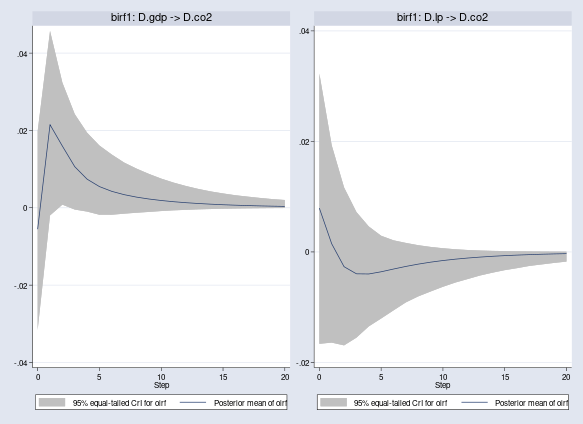
Clearly, the effects of the shocks to D.gdp and D.lp on D.co2 wear off after 20 quarters.
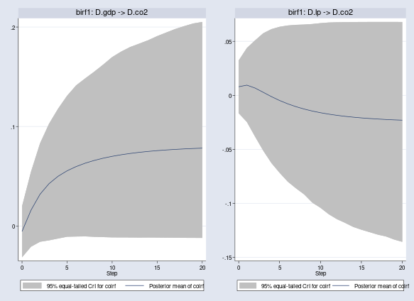
We also show the cumulative orthogonal IRFs, coirf, which are convenient for displaying the accumulating long-term shock effects.
. bayesirf cgraph (birf1 D.gdp D.co2 coirf) (birf1 D.lp D.co2 coirf)
Alternatively, we can show the cumulative orthogonal IRFs in table format by using the bayesirf ctable command.
. bayesirf ctable (birf1 D.gdp D.co2 coirf) (birf1 D.lp D.co2 coirf)
| (1) (1) (1) | ||
| Step | coirf Lower Upper | |
| 0 | -.005524 -.031529 .019887 | |
| 1 | .015962 -.020886 .054666 | |
| 2 | .031921 -.015899 .083129 | |
| 3 | .042553 -.014467 .10284 | |
| 4 | .04996 -.012635 .117914 | |
| 5 | .055443 -.010862 .130909 | |
| 6 | .059693 -.010626 .141337 | |
| 7 | .063087 -.010477 .148322 | |
| 8 | .065849 -.010923 .155024 | |
| 9 | .068122 -.0112 .162178 | |
| 10 | .070008 -.011505 .169777 | |
| 11 | .071581 -.011551 .175304 | |
| 12 | .072899 -.01158 .179913 | |
| 13 | .074008 -.0117 .183291 | |
| 14 | .074944 -.011603 .186745 | |
| 15 | .075737 -.011675 .19087 | |
| 16 | .07641 -.011786 .194462 | |
| 17 | .076983 -.011874 .198018 | |
| 18 | .077473 -.01194 .200903 | |
| 19 | .077892 -.011989 .203582 | |
| 20 | .078252 -.012025 .205119 | |
| (2) (2) (2) | ||
| Step | coirf Lower Upper | |
| 0 | .007935 -.016624 .032302 | |
| 1 | .009412 -.0247 .043826 | |
| 2 | .006742 -.038259 .050867 | |
| 3 | .002787 -.051265 .05746 | |
| 4 | .002787 -.051265 .05746 | |
| 5 | -.004791 -.071762 .063447 | |
| 6 | -.007885 -.07997 .064647 | |
| 7 | -.010504 -.086108 .065251 | |
| 8 | -.012708 -.091735 .065519 | |
| 9 | -.014557 -.099397 .066014 | |
| 10 | -.01611 -.104177 .066809 | |
| 11 | -.017417 -.110072 .067407 | |
| 12 | -.018518 -.114654 .067636 | |
| 13 | -.019448 -.118082 .067759 | |
| 14 | -.020235 -.121866 .067848 | |
| 15 | -.020904 -.124446 .067912 | |
| 16 | -.021473 -.126708 .067938 | |
| 17 | -.021959 -.129002 .067936 | |
| 18 | -.022374 -.130675 .067934 | |
| 19 | -.02273 -.133542 .067932 | |
| 20 | -.023035 -.135692 .06793 | |
bayesirf ctable reports posterior means (first column) and the lower and upper 95% credible bounds (second and third columns). After 20 quarters, one unit shock to the growth rate of gdp results in a 0.08-unit increase in the growth rate of co2, as given by the posterior mean estimate, and one unit shock to the growth rate of lp results in a 0.02-unit decrease in the growth rate of co2. On the other hand, the wide 95% credible bounds with significant mass on both sides of the zero line suggest that the effects to the shocks, especially that of D.lp on D.co2, are not that strong.
We can make more-specific conclusions by varying the credible-interval levels. For example, the 90% credible interval for D.gdp → D.co2 and 30% for D.lp → D.co2 do not include the zero after 20 quarters, indicating that the effect of D.gdp on D.co2 is positive with at least 90% probability and that the effect of D.lp on D.co2 is negative with at least 30% probability. Classical analysis based on confidence intervals does not provide such useful interpretations.
. bayesirf cgraph (birf1 D.gdp D.co2 coirf, clevel(90))
>                  (birf1 D.lp D.co2 coirf, clevel(30))
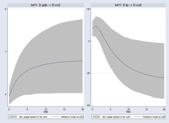
Although not strongly conclusive, the IRF results suggest that an increase of the growth rate of GDP causes an increase of the growth rate of CO2 emissions, which can be partially offset by an increase in labor productivity.
Bayesian forecasting
Finally, I want to illustrate Bayesian dynamic forecasting using the bayesfcast commands. In contrast to classical dynamic forecasts, which are based on point estimates, Bayesian forecasts consider the posterior predictive distributions at future time points.
We use bayesfcast compute to compute and save Bayesian forecasts as new variables in the dataset. For any given prefix, say, B_, the latter include posterior mean estimates B_*, posterior standard deviations B_*_sd, and lower and upper credible bounds B_*_lb and B_*_ub.
Below, we compute Bayesian forecasts starting from the first quarter of 2009 for 30 quarters into the future, thus reaching the end of the observed period.
. bayesfcast compute B_, dynamic(tq(2009q1)) step(30) rseed(17)
Then we use the bayesfcast graph command to plot the posterior mean forecasts for D.gdp and D.co2, along with their observed values.
. bayesfcast graph B_D_gdp, observed nodraw name(fcast_gdp)

. bayesfcast graph B_D_co2, observed nodraw name(fcast_co2)

. graph combine fcast_gdp fcast_co2, rows(1)
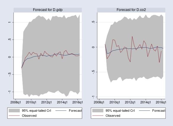
The dynamic forecasts are computed from the observed values of D.gdp, D.lp, and D.co2 only at the beginning of the forecast period (first quarter of 2009) and the quarter before (because we fit VAR(1)). The posterior mean estimates predict an initial increase in the growth rate of GDP and drop in the growth rate of CO2, followed by negligible growth rates for both. Unsurprisingly, the posterior mean forecasts cannot capture the observed fluctuations during the following 30 quarters—fluctuations caused by external factors not incorporated in the model.
The default 95% credible intervals include the observed values for D.gdp and D.co2 and are in fact quite wide. Bayesian results thus suggest significant forecasting uncertainty and overall weak prediction power of our simple model.
References
Baum, C. F., and S. Hurn. 2021. Environmental Econometrics Using Stata. College Station, TX: Stata Press.
Canova, F. 2007. Methods for Applied Macroeconomic Research. Princeton, NJ: Princeton University Press.
Grossman, G. M., and A. B. Krueger. 1993. Environmental impacts of a North American Free Trade Agreement. In The Mexico–U.S. Free Trade Agreement, ed. P. M. Garber, p. 13–54. Cambridge: MIT Press.
——. 1995. Economic growth and the environment. Quarterly Journal of Economics 110: 353–377.
— by Nikolay Balov
Principal Statistician and Software Developer


