

Stata's growing interoperability: The case of PyStata & Jupyter Notebook
When Stata 1.0 came out in 1985, it had 44 commands on a couple of 5¼-inch floppies. The only other software it interacted with was the DOS operating system on a PC. Things have changed—not just in terms of the plethora of commands and functions, or the multitude of platforms Stata can run on, but also in terms of extensibility and interoperability. Stata goes beyond Web awareness, the ability to import/export data, or plugins. It can now seamlessly interact, integrate, and interoperate with a growing number of popular software environments and programming languages.
Here are a few new interoperability capabilities in Stata 17:
- We introduced Python integration in Stata 16, or the ability to execute Python code from within Stata programs. We have enhanced PyStata, and now it also works the other way around—call Stata from Python, whether it is in Jupyter Notebook, Spyder, or PyCharm, all emerging development environments.
- We provide JDBC support that enables both import and export access to many databases, including Oracle, MySQL, Amazon Redshift, Snowflake, Microsoft SQL Server, and more.
- You can now embed Java code directly in do-files and ado-files, just like Mata or Python code. The Java code compiles on the fly.
- We also provide integration with H2O, an open-source artificial intelligence and machine-learning platform.
These integrations allow you to seamlessly and platform-agnostically (Windows, Mac, or Linux) pass around data, metadata, and results, and you can even display graphs.
We know it's a lot. So, in this note, we'll focus just on how you can run Stata from Jupyter Notebook.
pystata: A Python package for Stata
In Stata 17, Stata can be invoked from a standalone Python environment (like Jupyter Notebook, Spyder, or PyCharm) via a Python package called pystata. pystata provides two sets of tools:
- Three IPython (Interactive Python) magic commands:
- A suite of API functions for interacting with Stata from within Python.
With these tools, you can call Stata and Mata conveniently from various Python environments. See [P] PyStata module and pystata – Call Stata from Python for more details.
Calling Stata from Jupyter Notebook
Jupyter Notebook is a powerful and easy-to-use web application for interactive computing. It is widely used by researchers and scientists to share ideas and results. Jupyter Notebook can be easily and quickly installed.
Before calling Stata from Jupyter Notebook, we need to import and configure the pystata package to initialize Stata. There are a few ways to initialize Stata within a Python environment. For more information, see the pystata documentation on configuration.
Below, we use the first method listed in configuration. This method uses a Python module called stata_setup, which is available in the Python Package Index (PyPI). Suppose you have Stata installed in C:\Program Files\Stata17\ and you use the Stata/MP edition. Stata can be initialized as follows:
In [1]:
import stata_setup
stata_setup.config("C:/Program Files/Stata17", "mp")
   ___  ____  ____  ____  ____ ©
  /__    /   ____/   /   ____/      17.0
 ___/   /   /___/   /   /___/       MP—Parallel Edition

  Statistics and Data Science       Copyright 1985-2021 StataCorp LLC
                                    StataCorp
                                    4905 Lakeway Drive
                                    College Station, Texas 77845 USA
                                    800-STATA-PC        https://www.stata.com
                                    979-696-4600        [email protected]

 Stata license: 10-user 4-core network perpetual
 Serial number: 1
   Licensed to: Stata Developer
                StataCorp LLC

 Notes:
       1. Unicode is supported; see help unicode_advice.
       2. More than 2 billion observations are allowed; see help obs_advice.
       3. Maximum number of variables is set to 5,000; see help set_maxvar.

 .
If you get similar output for your edition of Stata, it means that everything is configured properly.
Run Stata using the %%stata magic command
Within Jupyter Notebook, you can use magic commands to access Stata and Mata. Magics are handy commands built into the IPython kernel that make it easy to perform particular tasks, for example, interacting Python's capabilities with the operating system or another programming language. The pystata package provides three magic commands, one of which is %%stata, which is used to execute Stata commands within Jupyter Notebook.
The Jupyter Notebook consists of a sequence of cells. In a cell, we put Stata commands underneath %%stata to direct the cell to call Stata. For example, the following code loads the auto dataset and summarizes the mpg (miles per gallon) variable. The Stata output is displayed underneath the cell.
In [2]:
%%stata
sysuse auto, clear
summarize mpg
 . sysuse auto, clear
 (1978 automobile data)

 . summarize mpg

     Variable |        Obs        Mean    Std. dev.       Min        Max
 -------------+---------------------------------------------------------
          mpg |         74     21.2973    5.785503         12         41

 .
The %%stata magic command provides a few arguments to control the execution of Stata's commands within the cell. With these arguments you can, for example, load data from Python into Stata, perform computations or estimations with Stata, and then pass Stata results back to Python, or vice versa.
In the following cell, we first run a linear regression and list the stored estimation results, or e-results, in e(). Then we store these results in Python as a dictionary named myeret.
In [3]:
%%stata -eret myeret
reg mpg price i.foreign
ereturn list
 . reg mpg price i.foreign

       Source |       SS           df       MS      Number of obs   =        74
 -------------+----------------------------------   F(2, 71)        =     23.01
        Model |  960.866305         2  480.433152   Prob > F        =    0.0000
     Residual |  1482.59315        71  20.8815937   R-squared       =    0.3932
 -------------+----------------------------------   Adj R-squared   =    0.3761
        Total |  2443.45946        73  33.4720474   Root MSE        =    4.5696

 ------------------------------------------------------------------------------
          mpg | Coefficient  Std. err.      t    P>|t|     [95% conf. interval]
 -------------+----------------------------------------------------------------
        price |   -.000959   .0001815    -5.28   0.000     -.001321    -.000597
              |
      foreign |
     Foreign  |   5.245271   1.163592     4.51   0.000     2.925135    7.565407
        _cons |   25.65058   1.271581    20.17   0.000     23.11512    28.18605
 ------------------------------------------------------------------------------

 . ereturn list

 scalars:
                   e(N) =  74
                e(df_m) =  2
                e(df_r) =  71
                   e(F) =  23.00749448574634
                  e(r2) =  .3932401256962295
                e(rmse) =  4.569638248831391
                 e(mss) =  960.8663049714787
                 e(rss) =  1482.593154487981
                e(r2_a) =  .3761482982510528
                  e(ll) =  -215.9083177127538
                e(ll_0) =  -234.3943376482347
                e(rank) =  3

 macros:
             e(cmdline) : "regress mpg price i.foreign"
               e(title) : "Linear regression"
           e(marginsok) : "XB default"
                 e(vce) : "ols"
              e(depvar) : "mpg"
                 e(cmd) : "regress"
          e(properties) : "b V"
             e(predict) : "regres_p"
               e(model) : "ols"
           e(estat_cmd) : "regress_estat"

 matrices:
                   e(b) :  1 x 4
                   e(V) :  4 x 4

 functions:
              e(sample)

 .
You can access specific elements of the dictionary in Python. For example, you can access the coefficients stored in e(b) by typing myeret[‘e(b)’].
In [4]:
myeret['e(b)']
 array([[-9.59034169e-04,  0.00000000e+00,  5.24527100e+00,
         2.56505843e+01]])
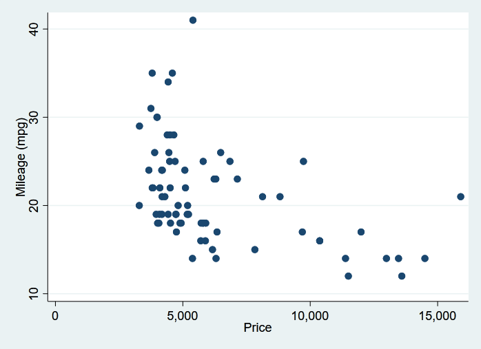
Stata graphs can also be directly displayed in Jupyter Notebook. Here we create a scatterplot of mpg against price.
In [5]:
%stata scatter mpg price
Call Mata using the %%mata magic command
The %%mata magic command is used to execute single lines of Mata code or multiple lines of Mata code at once. This is similar to executing Mata in a do-file. See [M-3] mata for more information about how to invoke Mata. For example, here is Mata code to create and display an identity matrix:
In [6]:
%%mata
/* function to create an nxn identity matrix */
real matrix id(real scalar n)
{
real scalar i
real matrix res
res = J(n, n, 0)
for (i=1; i<=n; i++) {
res[i,i] = 1
}
return(res)
}
/* create a 3x3 indentity matrix */
A = id(3)
A
 . mata
 ------------------------------------------------- mata (type end to exit) -----
 : /* function to create an nxn identity matrix */
 : real matrix id(real scalar n)
 > {
 >     real scalar i
 >     real matrix res
 >
 >     res = J(n, n, 0)
 >     for (i=1; i<=n; i++) {
 >         res[i,i] = 1
 >     }
 >     return(res)
 > }

 :
 : /* create a 3x3 indentity matrix */
 : A = id(3)

 : A
 [symmetric]
        1   2   3
     +-------------+
   1 |  1          |
   2 |  0   1      |
   3 |  0   0   1  |
     +-------------+

 : end
 -------------------------------------------------------------------------------
Interact with Stata using API functions
We can also interact with Stata from Python by using a suite of functions defined in the config and stata modules from the pystata Python package. We will demonstrate how to use these Application Programming Interface (API) functions to interact with Stata as an alternative to the %%stata magic command.
For example, we want to run a logistic regression on the NHANES II (Second National Health and Nutrition Examination Survey) dataset to determine how high blood pressure is related to age and weight.
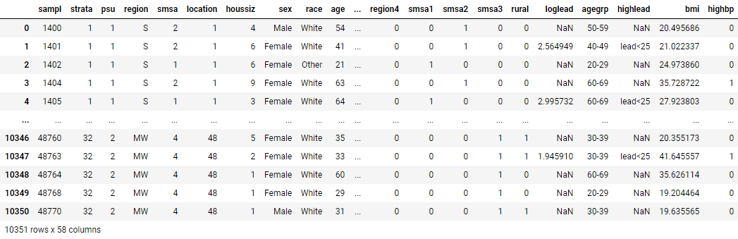
Suppose the original dataset is stored in a .csv file called nhanes2.csv, and it has been loaded into a pandas DataFrame named nhanes2 in Python. Here is how we pass this dataset into Stata:
In [7]:
import pandas as pd
import io
import requests
data = requests.get("https://www.stata.com/python/pystata18/misc/nhanes2.csv").content
nhanes2 = pd.read_csv(io.StringIO(data.decode('utf-8')))
nhanes2
Now, we import the stata module from pystata. Then, we call the pdataframe_to_data() function to load the dataset into Stata. Finally, we call the run() method to fit the logistic regression model. You can learn more about the many ways to load data from Python into Stata's current dataset in memory, and about pandas DataFrame, from Example2: Load data from Python.
In [8]:
from pystata import stata
stata.pdataframe_to_data(nhanes2, force=True)
stata.run('logistic highbp c.age##c.weight')
 Logistic regression                                    Number of obs =  10,351
                                                        LR chi2(3)    = 2381.23
                                                        Prob > chi2   =  0.0000
 Log likelihood = -5860.1512                            Pseudo R2     =  0.1689

 ------------------------------------------------------------------------------
       highbp | Odds ratio   Std. err.      z    P>|z|     [95% conf. interval]
 -------------+----------------------------------------------------------------
          age |   1.108531   .0080697    14.15   0.000     1.092827     1.12446
       weight |   1.081505    .005516    15.36   0.000     1.070748    1.092371
              |
        c.age#|
     c.weight |   .9992788   .0000977    -7.38   0.000     .9990873    .9994703
              |
        _cons |   .0002025   .0000787   -21.89   0.000     .0000946    .0004335
 ------------------------------------------------------------------------------
 Note: _cons estimates baseline odds.
After the estimation, we can use the get_ereturn() method to store the estimation results returned by the command in Python as a dictionary, say, myereturn. Here we display e-results e(b) and e(V) (coefficients and variance–covariance estimators, respectively).
In [9]:
myereturn = stata.get_ereturn()
myereturn['e(b)'], myereturn['e(V)']
(array([[ 1.03035513e-01, 7.83537342e-02, -7.21492384e-04,
         -8.50485078e+00]]),
 array([[ 5.29930771e-05, 3.50509317e-05, -6.97861002e-07,
         -2.69423163e-03],
        [ 3.50509317e-05, 2.60132664e-05, -4.74084051e-07,
         -1.94299575e-03],
        [-6.97861002e-07, -4.74084051e-07, 9.55811835e-09,
          3.50377699e-05],
        [-2.69423163e-03, -1.94299575e-03, 3.50377699e-05,
          1.50887842e-01]]))
For more details on calling Stata using API functions, check out Example5: Call Stata using API functions.
Final remarks
These are simple examples. The full power of Stata and Mata, including graphic capabilities, can now be unleashed from Python. For more details and examples see
- Jupyter Notebook with Stata
- Call Stata from Python
- Built-in magic commands
- Load data from Python
- Call Stata using API functions
We understand the importance of extensibility and interoperability. So in Stata 17, we enhanced PyStata, provided access to more databases, allowed integration with Java, and connected with H2O. We look forward to seeing you take advantage of the interoperabilities in the growing ecosystem we are building around Stata.
References
McDowell, A., A. Engel, J. T. Massey, and K. Maurer. 1981. Plan and operation of the Second National Health and Nutrition Examination Survey, 1976–1980. Vital and Health Statistics 1: 1–144.
Mckinney, W. 2010. Data Structures for Statistical Computing in Python. Proceedings of the 9th Python in Science Conference 56–61. (publisher link)
Péz, F., and B. E. Granger. 2007. IPython: A system for interactive scientific computing. Computing in Science and Engineering 9: 21–29. DOI:10.1109/MCSE.2007.53 (publisher link).
— Kreshna Gopal
Senior Computer Scientist & Software Developer
— Zhao Xu
Principal Software Engineer


