

In the spotlight: Intraclass correlations after multilevel survival models
As analysts, we like our data to be independent. Sometimes our data don't cooperate. Sometimes our data have groupings such that the observations within the groups are unlikely to be independent. For instance, you may have patients who were treated at the same hospital or students who attend the same school. One way to account for this lack of independence is to fit a multilevel survival model and include group-level random effects. Stata's mestreg command that was introduced in Stata 14 does just that.
Survival models are usually formulated using the proportional-hazards parameterization or using the accelerated failure-time (AFT) parameterization, both of which are available with mestreg. One of the advantages of the AFT metric, when fitting multilevel models, is that the variances of the random effects at different grouping levels can be interpreted as variance components of the log-time. This is possible because, in the AFT metric, we model the log-time as a linear combination of random effects (and covariates). We can use those variances and the variance of the residuals to compute intraclass correlations for the log-time.
To demonstrate, I use an example based on the study of the survival probability of scrub-jay birds from Fox et al. (2006). The authors used a dataset on survival of scrub-jays collected over 35 years, where several territories were censused periodically, and data on birth cohort (year), territory, and parents were recorded, among other variables. Birds tend to stay in a territory, so mother and father have a constant territory throughout the years, although mating couples vary among years.
Fox et al. (2006) fit several two-level Weibull models to the data with fixed effects for the cohort and with random effects on territory, maternal family, or paternal family. They didn't fit multilevel models with more than two levels, perhaps because of the software limitations at that time. I use a fictional dataset with only five cohorts to demonstrate several multilevel models we could fit to the data. Observations are censored, assuming that many birds were alive at the end of this fictional five-year study.
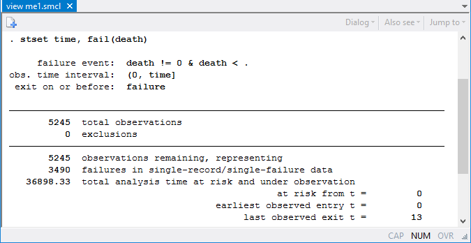
We use stset to declare our survival-time data: time records time-to-death (or time-to-censoring) of birds in years, and death is a failure indicator of birds' death or censoring.
First, let's fit a Weibull model with dummy variables for each of the five cohorts (years) and random effects on territory.
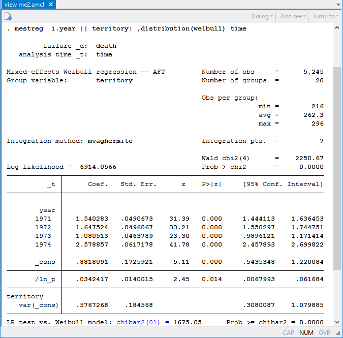
The main part of the table shows the coefficients for the fixed part of the model. The baseline cohort (reference category) is 1970. The mean survival time, assuming zero random effects, can be computed with predict, mean conditional(fixedonly).
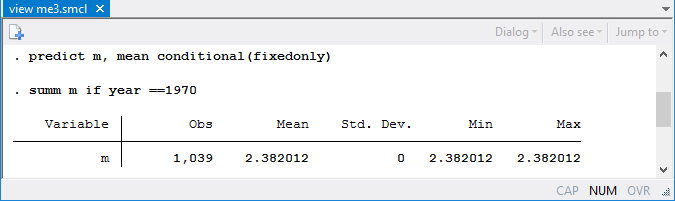
The mean survival for birds in the baseline cohort (assuming zero random effects) is 2.38 years.
Based on our estimate of the coefficient for the dummy for year 1971, the mean survival of birds born in 1971 is exp(1.54)=4.67 times longer than those born in 1970. Similarly for other cohorts, the mean survival times are 5.19, 2.95, and 13.18 times longer than for the baseline cohort. The best year (that is, the cohort with the largest mean survival time) is 1974. The likelihood-ratio test, reported at the bottom of the mestreg ouput, indicates that the model with random effects for territory fits better than the model without random effects. Random effects on territory have a variance equal to 0.58.
Now, let's fit a model with random effects on mother.
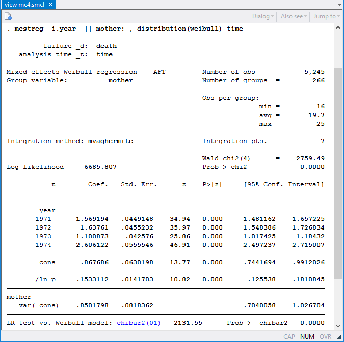
The variance of random effects on mother is estimated to be 0.85. Fox et al. (2006) mentioned that the mother effect is confounded with the territory effect. Because mothers are nested within territories, we can fit a three-level nested model:
Now that we have accounted for the variability due to territory, the variability due to mother is lower.
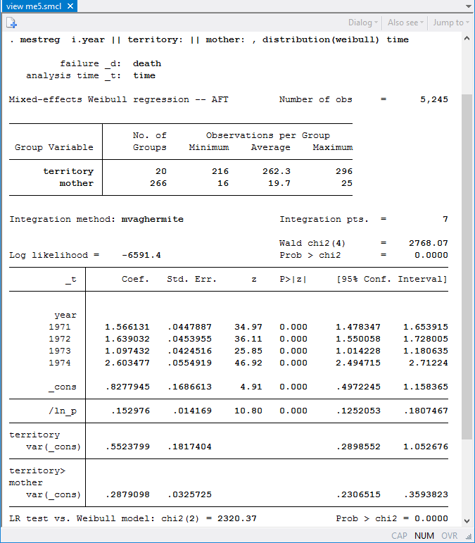
The model above can be written as follows in the AFT parameterization,
$$ ln(T) = xb + u_{i} + u_{ij} + \epsilon_{ijk} $$
where level-3 (territory) and level-2 (mother nested within territory) random effects, \(u_{i}\) and \(u_{ij}\), are normally distributed with zero means and with variances \(\sigma^2_3\) and \(\sigma^2_2\). \(\epsilon_{ijk}\) are the error terms; their variance, \(\sigma^2_1\), is the variance component at the individual level. For AFT models in general, \(\epsilon_{ijk}\) are assumed to be independent and identically distributed, and their distribution depends on the model we are fitting. See Rodríguez (2010) for a discussion of the distribution of the errors for different AFT survival models. In the case of the Weibull distribution, \(\epsilon_{ijk}\) follow the Gumbell distribution, and their variance is \(\pi^2/(6\times p^2)\), where \(p\) is the ancillary parameter of the Weibull distribution. We can compute the residual variance using the estimate of the log of \(p\) stored in _b[ln_p:_cons] by mestreg,
    . display _pi^2/(6 *exp(2*_b[ln_p:_cons]))
    1.2113656
From the values obtained above, we can construct the following table of variance components:
| Variance component | |||
|---|---|---|---|
| Level | Grouping variable | Symbol | Estimate |
| 1 | individual (_n) | \(\sigma^2_1\) | 1.2113656 |
| 2 | mother<territory | \(\sigma^2_2\) | 0.2879098 |
| 3 | territory | \(\sigma^2_3\) | 0.5523799 |
We can use these values to compute intraclass correlations (ICCs). For example, we can obtain the formulas for ICCs from the Methods and formulas section in the [ME] mixed postestimation entry.
Level-3 (territory) ICC: \(\rho^{(3)} = \sigma^2_3/(\sigma^2_1 + \sigma^2_2 + \sigma^2_3)\)
Level-2 (mother) ICC: \(\rho^{(2)} = (\sigma^2_2 + \sigma^2_3)/(\sigma^2_1 + \sigma^2_2 + \sigma^2_3)\)
We can compute ICCs manually using the values of variance components from the table, or we can use nlcom:
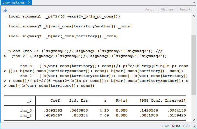
The correlation between log survival-times for birds in the same territory is 0.27 with a 95% CI of [0.14, 0.40], whereas the correlation between log survival-times for birds with the same mother (and therefore also in the same territory) is 0.41 with a 95% CI of [0.31, 0.51]. We can also apply transformations as described in Methods and formulas in [ME] mixed postestimation to ensure that the confidence limits are always between zero and one.
References
Fox, G. A., B. E. Kendall, J. W. Fitzpatrick, and G. E. Woolfenden. 2006. Consequences of heterogeneity in survival probability in a population of Florida scrub-jays. Journal of Animal Ecology 75: 921–927.
Rodríguez, G. 2010. Parametric Survival Models. http://data.princeton.edu/pop509/ParametricSurvival.pdf.
—Isabel Canette
Principal Mathematician and Statistician, StataCorp LP


