Power analysis for comparison of proportions

Let's see it work

Comparisons of proportions

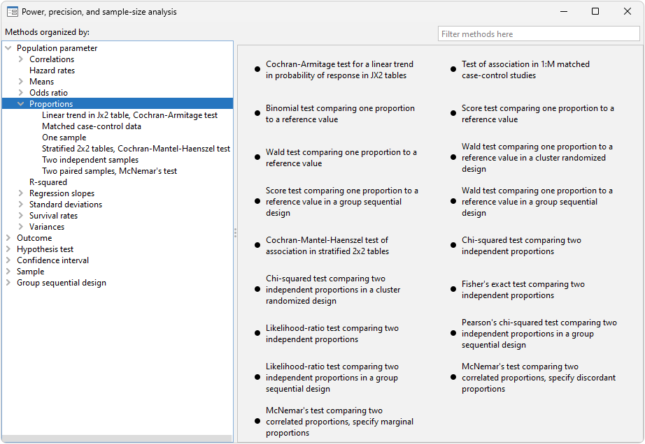
Stata's power suite provides three methods for classical tests of proportions and three methods for tests based on contingency tables. To see what is available (and for point-and-click analysis), go to the menu Statistics > Power, precision, and sample size and under Population parameter, select Proportions. For one of the classical proportion tests, select One sample, Two independent samples, or Two paired samples, McNemar's test.

power oneproportion estimates sample size, power, and effect size for a test comparing one proportion to a reference value. You can choose between a score test and a Wald test; the small-sample binomial test is also available for power estimation. Additionally, you can apply a continuity correction.

power twoproportions estimates sample size, power, and effect size for a test comparing two independent proportions. When estimating effect size, you can choose to report the effect size as the difference between the experimental-group proportion and the control-group proportion, the ratio of the experimental-group proportion and the control-group proportion, or the odds ratio. You can incorporate unbalanced designs and compute the sample size of one group given the other. Additionally, you can choose between Pearson's chi-squared test and a likelihood-ratio test; Fisher–Irwin's exact conditional test is also available for power estimation.

power pairedproportions estimates sample size, power, and effect size for a test comparing two proportions from paired samples. You can estimate sample-size and power by specifying either discordant or marginal proportions; effect sizes can be estimated only with discordant proportions. Effect sizes can be specified as a difference in proportions or a ratio of proportions; when working with marginal proportions, you can also specify the effect size as an odds ratio.

In addition, Stata's power command performs power analysis for tests of proportions based on contingency tables and for classical comparisons of proportions accounting for cluster randomized designs.

Suppose we want to investigate whether aspirin is effective in reducing the mortality rate due to heart attacks. Also, suppose previous studies have found that the proportion of deaths due to heart attacks is 0.02 for individuals who don't take aspirin and 0.001 for those who do. We suspect the proportion might be higher for those who do. So we examine the power we can obtain for sample sizes of 1500 through 3000 for hypothesized proportions of 0.001 through 0.004.

We type

. power twoproportions 0.02 (0.001 0.002 0.003 0.004), n(1500 2000 2500 3000) graph

Above, we specified hypothesized proportions of death due to heart attacks for individuals who take aspirin. We could have instead specified the hypothesized difference in proportions between aspirin users and nonusers, the ratio of the proportions, or the odds ratio.

Now suppose that we're interested in calculating the sample sizes required to detect those different proportions at power levels of 0.8 and 0.9. We would type

. power twoproportions 0.02 (0.001 0.002 0.003 0.004), power(0.8 0.9) graph

For a given level of power, the required sample size increases as the hypothesized proportion of deaths for aspirin users (experimental group) increases.

We can also investigate the smallest detectable difference in proportions of death for aspirin users and nonusers, given a range of sample sizes and levels of power. Our alternative hypothesis is that the proportion of deaths for aspirin users is lower than the proportion for nonusers, so we specify the direction of the effect as well. (The default assumes the proportion for the experimental group is greater than that for the control group.)

. power twoproportions 0.02, n(1500 2000 2500 3000) power(0.8 0.9) direction(lower) graph

We get a plot of the estimated proportions for aspirin users that correspond to the smallest detectable differences. We can instead plot the effect sizes (difference between the proportions for users and nonusers) by specifying y(delta) within the graph() option:

. power twoproportions 0.02, n(1500 2000 2500 3000) power(0.8 0.9) direction(lower) graph(y(delta))

In this graph, the effect size is calculated as (proportion for aspirin users - 0.02). Because the estimated proportions are smaller for aspirin users than nonusers, we get a series of negative values.