1 item has been added to your cart.
| Title | How can I remove rows or columns from a table generated with collect, table, or dtable? | |
| Author | Gabriela Ortiz, StataCorp |
When creating tables of results, you may find that you want to remove certain rows or columns. To do so, you need to know how to refer to the results that are being collected; the key is to identify the dimensions and the levels for the specific results we want. In this FAQ, we will demonstrate how to modify the rows and columns after creating a table with collect, table, and dtable. The FAQ is organized as follows:
Suppose we want to create a table of estimation results after fitting a linear regression model. First, we collect the estimation results with the collect prefix, and then we lay out our table:
. collect clear

. webuse nhanes2l, clear
(Second National Health and Nutrition Examination Survey)

. collect: regress bpsystol age weight i.sex
| Source | SS df MS | Number of obs = 10,351 | F(3, 10347) = 1501.75 |
| Model | 1709209.9 3 569736.633 | Prob > F = 0.0000 | |
| Residual | 3925460.13 10,347 379.381476 | R-squared = 0.3033 | Adj R-squared = 0.3031 |
| Total | 5634670.03 10,350 544.412563 | Root MSE = 19.478 |
| bpsystol | Coefficient Std. err. t P>|t| [95% conf. interval] | |
| age | .6374325 .0111334 57.25 0.000 .6156088 .6592562 | |
| weight | .4170339 .013474 30.95 0.000 .3906221 .4434456 | |
| sex | ||
| Female | .8244702 .4140342 1.99 0.046 .0128832 1.636057 | |
| _cons | 70.13615 1.187299 59.07 0.000 67.80881 72.46348 | |
| Coefficient 95% CI df 95% lower bound p-value Std. error 95% upper bound t |t| Standardized coefficient | ||
| Age (years) | .6374325 .6156088 .6592562 10347 .6156088 0.000 .0111334 .6592562 57.25 57.25 .4702977 | |
| Weight (kg) | .4170339 .3906221 .4434456 10347 .3906221 0.000 .013474 .4434456 30.95 30.95 .2744714 | |
| Male | 0 0 0 | |
| Female | .8244702 .0128832 1.636057 10347 .0128832 0.046 .4140342 1.636057 1.99 1.99 .0176462 | |
| Intercept | 70.13615 67.80881 72.46348 10347 67.80881 0.000 1.187299 72.46348 59.07 59.07 | |
For models with a single outcome variable, we can lay out our table by specifying dimensions colname and result; in this example, we placed levels of colname on the rows and levels of result on the columns of the table. The name colname refers to the column names of the returned matrix e(b), and it identifies the independent variables in our model. The third row in the table corresponds to Male, the base level for sex; we can specify that base levels not be shown with the following setting:
. collect style showbase off
The dimension result identifies the results returned in e() and r(), such as the coefficients, confidence intervals, and model statistics. We have more results than we’d like in our table. Suppose we only want to include the coefficients and confidence intervals. We can list the levels of dimension result to see how to refer to these results:
. collect levelsof result

Collection: default
 Dimension: result
    Levels: F N _r_b _r_ci _r_df _r_lb _r_p _r_se _r_ub _r_z _r_z_abs beta cmd
            cmdline depvar df_m df_r estat_cmd ll ll_0 marginsok model mss
	    predict properties r2 r2_a rank rmse rss title vce
It may not be obvious from the result names which ones we want, so instead we list the levels with their labels. It’s good practice to add the all option so that all levels get listed, even those without a label:
. collect label list result, all

  Collection: default
   Dimension: result
       Label: Result
Level labels:
           F  F statistic
           N  Number of observations
        _r_b  Coefficient
       _r_ci  __LEVEL__% CI
       _r_df  df
       _r_lb  __LEVEL__% lower bound
        _r_p  p-value
       _r_se  Std. error
       _r_ub  __LEVEL__% upper bound
        _r_z  t
    _r_z_abs  |t|
        beta  Standardized coefficient
         cmd  Command
     cmdline  Command line as typed
      depvar  Dependent variable

(output omitted)
We now spot _r_b for coefficients and _r_ci for confidence intervals, and we include only these levels of the dimension result.
. collect layout (colname) (result[_r_b _r_ci])

Collection: default
      Rows: colname
   Columns: result[_r_b _r_ci]
   Table 1: 5 x 2
| Coefficient 95% CI | ||
| Age (years) | .6374325 .6156088 .6592562 | |
| Weight (kg) | .4170339 .3906221 .4434456 | |
| Male | 0 | |
| Female | .8244702 .0128832 1.636057 | |
| Intercept | 70.13615 67.80881 72.46348 | |
In fact, if you find yourself specifying the same levels of a dimension each time, you can set the levels to be automatically displayed. For example, below we specify that only the coefficients and confidence intervals be displayed whenever we list the dimension result:
. collect style autolevels result _r_b _r_ci, clear
And now if we simply list the dimension result, we’ll only get those two results:
. collect layout (colname) (result)

Collection: default
      Rows: colname
   Columns: result
   Table 1: 4 x 2
| Coefficient 95% CI | ||
| Age (years) | .6374325 .6156088 .6592562 | |
| Weight (kg) | .4170339 .3906221 .4434456 | |
| Female | .8244702 .0128832 1.636057 | |
| Intercept | 70.13615 67.80881 72.46348 | |
The automatic level specification applies only to this collection, but you can use collect style save to save these style settings and later apply them to another collection. Learn more about automatic levels in FAQ: What are the autolevels of a dimension in a table (collection)? and in the documentation for collect style autolevels.
When creating tables with the table command, we are simultaneously specifying the statistics we want displayed and the layout of our table. With table as well, we may find that we want to remove rows or columns. For example, consider this table with the percentage of males and females in each age group who have had a heart attack.
. table (agegrp) (sex heartatk), statistic(percent, across(heartatk)) sformat("%s%%") missing
| Sex | ||
| Male Female Total | ||
| Prior heart attack Prior heart attack Prior heart attack | ||
| No heart attack Had heart attack Total No heart attack Had heart attack . Total No heart attack Had heart attack . Total | ||
| Age group | ||
| 20–29 | 100.00% 100.00% 99.92% 0.08% 100.00% 99.96% 0.04% 100.00% | |
| 30–39 | 99.74% 0.26% 100.00% 99.65% 0.23% 0.12% 100.00% 99.69% 0.25% 0.06% 100.00% | |
| 40–49 | 98.03% 1.97% 100.00% 98.64% 1.21% 0.15% 100.00% 98.35% 1.57% 0.08% 100.00% | |
| 50–59 | 92.36% 7.64% 100.00% 96.66% 3.34% 100.00% 94.66% 5.34% 100.00% | |
| 60–69 | 86.56% 13.44% 100.00% 94.57% 5.43% 100.00% 90.73% 9.27% 100.00% | |
| 70+ | 83.48% 16.52% 100.00% 92.01% 7.99% 100.00% 88.13% 11.87% 100.00% | |
| Total | 93.53% 6.47% 100.00% 97.06% 2.91% 0.04% 100.00% 95.38% 4.60% 0.02% 100.00% | |
By default, table will report totals for each category. We specified the missing option to include any observations with a missing value and the sformat() option to display a percent sign next to the percentages.
The table seems too wide for our taste, and we now decide to omit the columns for the totals and missing values. Also, suppose that we’re interested only in people 40 and older. First, we’ll check the current layout specification with collect layout, and then we’ll modify the contents of the table.
. collect layout

Collection: Table
      Rows: agegrp
   Columns: sex#heartatk
    Tables: result
   Table 1: 8 x 11

(output omitted)
We see that the dimensions for the rows and columns correspond to the variables we specified in the parentheses. The dimension result identifies the requested statistics, which in our case is just percent. You can type collect dims to see what other dimensions we have in this collection.
We can select the levels of heartatk and agegrp that we want to include in our table, but we need to know what level refers to the 40s, 50s, and other age groups. Below, we list the levels of the dimensions and their labels, if there are any.
. collect label list sex, all

  Collection: Table
   Dimension: sex
       Label: Sex
Level labels:
          .m  Total
           1  Male
           2  Female

. collect label list agegrp, all

  Collection: Table
   Dimension: agegrp
       Label: Age group
Level labels:
          .m  Total
           1  20–29
           2  30–39
           3  40–49
           4  50–59
           5  60–69
           6  70+

. collect label list heartatk, all

  Collection: Table
   Dimension: heartatk
       Label: Prior heart attack
Level labels:
           .
          .m  Total
           0  No heart attack
           1  Had heart attack
The variable labels are used as the dimension labels; for example, the variable label for agegrp is “Age group”. The levels of each dimension are simply the numeric values, and the labels are obtained from the value labels. The one level you may not recognize is .m, which corresponds to the Total category. The level . is the category for missing values.
Now we know how to specify the levels of sex, agegrp, and heartatk that we want to include. Below, we include the age groups from 40 and above, and we omit the total and missing categories:
. collect layout (agegrp[3 4 5 6]) (sex[1 2]#heartatk[0 1]) (result)

Collection: Table
      Rows: agegrp[3 4 5 6]
   Columns: sex[1 2]#heartatk[0 1]
    Tables: result
   Table 1: 5 x 4
| Sex | ||
| Male Female | ||
| Prior heart attack Prior heart attack | ||
| No heart attack Had heart attack No heart attack Had heart attack | ||
| Age group | ||
| 40–49 | 98.03% 1.97% 98.64% 1.21% | |
| 50–59 | 92.36% 7.64% 96.66% 3.34% | |
| 60–69 | 86.56% 13.44% 94.57% 5.43% | |
| 70+ | 83.48% 16.52% 92.01% 7.99% | |
Now we have just the categories of interest, but our table header would look better if we hide the dimension labels for sex and heartatk:
. collect style header sex heartatk, title(hide)

. collect preview
| Male Female | ||
| No heart attack Had heart attack No heart attack Had heart attack | ||
| Age group | ||
| 40–49 | 98.03% 1.97% 98.64% 1.21% | |
| 50–59 | 92.36% 7.64% 96.66% 3.34% | |
| 60–69 | 86.56% 13.44% 94.57% 5.43% | |
| 70+ | 83.48% 16.52% 92.01% 7.99% | |
That’s much better.
When creating tables with the dtable command, we can specify the levels of factor variables that we want to include, but there still may be rows or columns that we wish to omit. For example, below we look at the percentage of individuals who have diabetes and those who have had a heart attack in each region of the United States.
. dtable age weight i.sex i.diabetes i.heartatk, by(region, nototals)
| Region |
| NE MW S W |
| N 2,096 (20.2%) 2,774 (26.8%) 2,853 (27.6%) 2,628 (25.4%) |
| Age (years) 47.816 (17.017) 46.528 (17.376) 48.191 (16.864) 47.838 (17.535) |
| Weight (kg) 71.646 (14.922) 72.050 (15.340) 72.035 (15.655) 71.787 (15.393) |
| Sex |
| Male 1,018 (48.6%) 1,310 (47.2%) 1,332 (46.7%) 1,255 (47.8%) |
| Female 1,078 (51.4%) 1,464 (52.8%) 1,521 (53.3%) 1,373 (52.2%) |
| Diabetes status |
| Not diabetic 1,997 (95.3%) 2,648 (95.5%) 2,692 (94.4%) 2,513 (95.6%) |
| Diabetic 98 (4.7%) 125 (4.5%) 161 (5.6%) 115 (4.4%) |
| Prior heart attack |
| No heart attack 2,018 (96.3%) 2,652 (95.6%) 2,722 (95.4%) 2,481 (94.4%) |
| Had heart attack 77 (3.7%) 121 (4.4%) 131 (4.6%) 147 (5.6%) |
I’m interested only in the percent of individuals with a prior heart attack or diabetes, so I omit the other categories below. Both diabetes and heartatk are binary variables, with a value of 1 indicating that the individual has the condition or disease, so we type
. dtable age weight i.sex 1.diabetes 1.heartatk, by(region, nototals)
| Region |
| NE MW S W |
| N 2,096 (20.2%) 2,774 (26.8%) 2,853 (27.6%) 2,628 (25.4%) |
| Age (years) 47.816 (17.017) 46.528 (17.376) 48.191 (16.864) 47.838 (17.535) |
| Weight (kg) 71.646 (14.922) 72.050 (15.340) 72.035 (15.655) 71.787 (15.393) |
| Sex |
| Male 1,018 (48.6%) 1,310 (47.2%) 1,332 (46.7%) 1,255 (47.8%) |
| Female 1,078 (51.4%) 1,464 (52.8%) 1,521 (53.3%) 1,373 (52.2%) |
| Diabetes status |
| Diabetic 98 (4.7%) 125 (4.5%) 161 (5.6%) 115 (4.4%) |
| Prior heart attack |
| Had heart attack 77 (3.7%) 121 (4.4%) 131 (4.6%) 147 (5.6%) |
In fact, I’m interested only in the West and Northeastern regions, but I can’t specify the levels of the by() variable with dtable. The first step is to check which dimensions are being used to lay out the table:
. collect layout

Collection: DTable
      Rows: var
   Columns: region#result
   Table 1: 10 x 4

(output omitted)
I also want to move the sample size to the last row of the table and reorder the regions, so I’m going to list the levels of var and the labels for region to see how to refer to the levels.
. collect levelsof var

Collection: DTable
 Dimension: var
    Levels: _N _hide age weight 1.sex 2.sex 1.diabetes 1.heartatk

. collect label list region

  Collection: DTable
   Dimension: region
       Label: Region
Level labels:
          .m  Total
           1  NE
           2  MW
           3  S
           4  W
We can use var[_N] to refer to the sample size and the numeric values of region to specify the regions we want. Below, we lay out our table with the two regions we are interested in, and we place _N after all the variables:
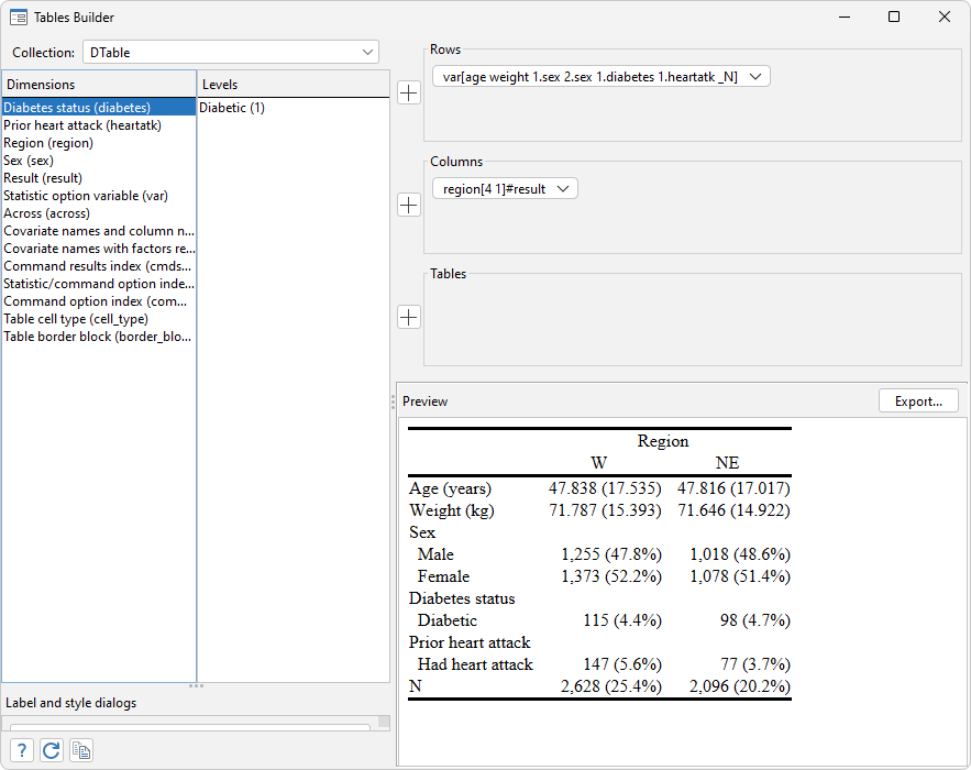
. collect layout (var[age weight i.sex 1.diabetes 1.heartatk _N]) (region[4 1]#result)

Collection: DTable
      Rows: var[age weight i.sex 1.diabetes 1.heartatk _N]
   Columns: region[4 1]#result
   Table 1: 10 x 2
| Region |
| W NE |
| Age (years) 47.838 (17.535) 47.816 (17.017) |
| Weight (kg) 71.787 (15.393) 71.646 (14.922) |
| Sex |
| Male 1,255 (47.8%) 1,018 (48.6%) |
| Female 1,373 (52.2%) 1,078 (51.4%) |
| Diabetes status |
| Diabetic 115 (4.4%) 98 (4.7%) |
| Prior heart attack |
| Had heart attack 147 (5.6%) 77 (3.7%) |
| N 2,628 (25.4%) 2,096 (20.2%) |
I specified region 4 before region 1 so that we have the West followed by the Northeast.
To learn more about the concepts of a collection and how the collect system works, read [TABLES] Intro 2.
In addition to creating your tables with the collect commands shown above, you can create them with the Tables Builder, shown below. See [TABLES] Tables Builder to learn more.