1 item has been added to your cart.

How can I customize my table to add cell shading and bold formatting and to underline text?

Suppose we have created the following table with baseline characteristics for the auto7 dataset,

Table 1.

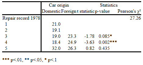
with the following code,

. clear all

. webuse auto7

. table (rep78) (foreign), stat(mean mpg) nototals

. table (rep78[3 4 5]), command(p2=r(p): ttest mpg, by(foreign)) nototals append

. collect, tags(rep78[_hide]):tabulate rep78 foreign, chi2

. collect stars p2 0.01 "***" 0.05 "**" .1 "*" , attach(p2) shownote

. collect layout (rep78[_hide 1 2 3 4 5]) (foreign result[t p2 chi2])

. collect style cell rep78#foreign, nformat(%4.1f)

. collect style cell result[p2], nformat(%5.3f) halign(left)

. collect style cell result[t chi2], nformat(%5.2f)

. collect style header result, title(label)

. collect label dim result "Statistics", modify

. collect label levels result "p2" "p-value"

. collect preview

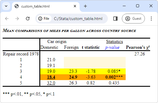
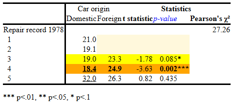
How can we customize the table so that it looks like the following?

Table 2.

Our goal is to demonstrate some common style changes you will likely want to make to your tables, such as adding a background color, formatting text as bold, or underlining your text. Note that some of the changes we’ll make are not supported by the Stata Markup and Control Language, which means they won’t be reflected when viewing the table in the Results window (more details can be found in FAQ: Why can't I observe the style changes (background shading, font, etc.) in my table in the Results window?); however, the style changes will be reflected in the Tables Builder and in the HTML file that we’ll export our table to. The table screenshots you’ll see below were taken from the Tables Builder.

This table shows the mean of the variable mpg (miles per gallon) for each combination of the levels of rep78 and foreign. For each category of rep78, we also performed a t test on the equality of mpg across foreign and domestic cars; we included the resulting t statistics and p-values in our table, too. In the last column, we included Pearson’s \(\chi^2\) test for a two-way tabulation between rep78 and foreign.

We don’t have any foreign cars with rep78 = 1 or rep78 = 2, so we highlight these empty cells with the color cornsilk. We also shade the two rows for which the t tests are significant, with different colors depending on the level of statistical significance. We find the strongest evidence of a statistically significant difference in the means when rep78 = 4, so we format the values for that category as bold. Additionally, we underline the minimum and maximum of the mean mpg values. For the dimension result, we underline the dimension label “Statistics” and format the labels for two levels as bold and the other (p-value) as blue and italic.

Customizing the body of the table

We can change the appearance style for our cells with the command collect style cell. The option shading(background()) allows us to specify the background color. We don’t have any foreign cars with rep78 = 1 or rep78 = 2, so we highlight cells in these missing categories. Additionally, we highlight the row with .01 < p < .1 yellow and the row with p < .01 orange. We can apply these background colors only to the intended cells by specifying the proper tags with collect style cell. For example, rep78[1 2]#foreign[1] refers to cells for which foreign = 1 and rep78 = 1 or rep78 = 2; rep78[3]#foreign refers to cells with rep78 = 3 for all levels of foreign.

. collect style cell rep78[1 2]#foreign[1] rep78[1 2]#result[t p2], shading(background(cornsilk))

. collect style cell rep78[3]#foreign rep78[3]#result[t p2], shading(background(yellow))

. collect style cell rep78[4]#foreign rep78[4]#result[t p2], shading(background(orange))

Next, we underline the minimum and maximum of the mean mpg values with the font(,underline(single)) option for collect style cell. The maximum value, 32.0, can be identified with the tag rep78[5]#foreign[0], and the minimum can be identified with rep78[4]#foreign[0].

. collect style cell rep78[5]#foreign[0], font(,underline(single))

. collect style cell rep78[4]#foreign[0], font(,underline(single))

We find the strongest evidence of a statistically significant difference in means when rep78 = 4, so we format the means and p-value as bold with option font(,bold); rep78[4]#foreign identifies the means and rep78[4]#result[p2] identifies the p-value.

. collect style cell rep78[4]#foreign rep78[4]#result[p2],font(, bold)

Now that we've made these style changes, the obtained table can be viewed in the Tables Builder (type db tables to open).

Table 3.

Similarly, the other tables in this FAQ can be viewed in this way.

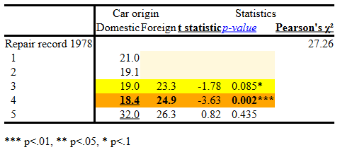
We're close to obtaining the table we want; we just need to customize the table headers, which we do next.

Customizing table headers

We first make the column header for the p-value blue and italic with option font(,color(blue) italic). We can refer to this cell with the tag cell_type[column-header]#result[p2]. The dimension cell_type divides the table into four sections: corner, column-header, row-header, and item. item refers to the body of the table. The tag cell_type[column-header] refers to all column headers, so we interact it with result[p2] to modify only the column header for the p-value. You can type collect dims to see all dimensions in the collection and collect levelsof cell_type to see all levels in the dimension cell_type.

. collect style cell cell_type[column-header]#result[p2],font(,color(blue) italic)

We cannot format the other two statistics tags in the same way, namely,

. collect style cell cell_type[column-header]#result[t], font(,bold)

. collect style cell cell_type[column-header]#result[chi2], font(,bold)

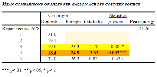
because changing the first level style will change the dimension style and thus make the label “Statistics” bold, too, as shown below,

Table 4.

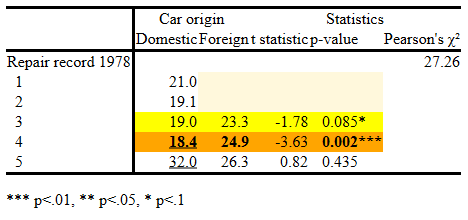
Similarly, if we try to underline the “Statistics” label with the following code,

. collect style cell cell_type[column-header]#result, font(, underline)

all the levels of the dimension result will be underlined.

Table 5.

One solution for this is to create another dimension that has the same label “Statistics” and add that dimension to the collect layout specification. For example, we created a dimension called stat and tagged all items in our collection with level _hide of dimension stat. Additionally, we hide the title for dimension result with collect style header result, title(hide). Then, we label dimension stat “Statistics” and interact stat with dimension result in our layout.

. collect style header result, title(hide)

. collect addtags stat[_hide]

. collect label dim stat "Statistics"

. collect layout (rep78[_hide 1 2 3 4 5]) (foreign stat#result[t p2 chi2])

The resulting table will no longer have the label “Statistics” formatted as bold because the bold formatting we previously specified was applied to the column header of dimension result.

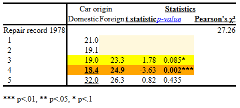
Table 6.

We can now add the underline to the stat[_hide] tag while removing the underline for the result dimension.

. collect style cell cell_type[column-header]#stat[_hide], font(, underline)

. collect style cell cell_type[column-header]#result, font(, nounderline)

To finish customizing this table and achieve the style we want, we need to make a few adjustments to the cell margins and alignment. We also add a title and format it with collect style title.

. collect style cell rep78, halign(center)

. collect style cell foreign[0], margin(right, width(.2in))

. collect style cell result[t],margin(right, width(.1in)) margin(left, width(.1in))

. collect style cell result[p2] ,margin(right, width(.1in)) margin(left, width(.1in))

. collect title "Mean comparisons of miles per gallon across country source"

. collect style title, font(,variant(smallcaps) italic bold)

. collect export custom_table.html, replace

The collect export command exports the table from Stata to an HTML file called custom_table.html.