
1 item has been added to your cart.
| Title | How to insert a customized statistic in an existing table by creating a new column or a new row | |
| Author | Mia Lv, StataCorp |
Frequently, researchers desire to customize their tables by incorporating new elements. Often, these new items need to be placed in a new row or column. How can this be achieved? Follow these steps:
In this example, we initially create a table of descriptive statistics with dtable; we wish to add a p-value obtained after fitting a logistic regression model. Here is our initial code:
. clear all

. sysuse auto
(1978 automobile data)

. dtable trunk mpg i.rep78, by(foreign) column(by(hide))
The table appears as
| Domestic Foreign Total |
| N 52 (70.3%) 22 (29.7%) 74 (100.0%) Trunk space (cu. ft.) 14.750 (4.306) 11.409 (3.217) 13.757 (4.277) Mileage (mpg) 19.827 (4.743) 24.773 (6.611) 21.297 (5.786) Repair record 1978 1 2 (4.2%) 0 (0.0%) 2 (2.9%) 2 8 (16.7%) 0 (0.0%) 8 (11.6%) 3 27 (56.2%) 3 (14.3%) 30 (43.5%) 4 9 (18.8%) 9 (42.9%) 18 (26.1%) 5 2 (4.2%) 9 (42.9%) 11 (15.9%) |
Now we would like to include a p-value corresponding to a hypothesis test. We want to place the p-value on the row for level 1 of “Repair record 1978”, creating a new column on the far right.
| Domestic Foreign Total p-value |
| N 52 (70.3%) 22 (29.7%) 74 (100.0%) Trunk space (cu. ft.) 14.750 (4.306) 11.409 (3.217) 13.757 (4.277) Mileage (mpg) 19.827 (4.743) 24.773 (6.611) 21.297 (5.786) Repair record 1978 1 2 (4.2%) 0 (0.0%) 2 (2.9%) 0.0005 2 8 (16.7%) 0 (0.0%) 8 (11.6%) 3 27 (56.2%) 3 (14.3%) 30 (43.5%) 4 9 (18.8%) 9 (42.9%) 18 (26.1%) 5 2 (4.2%) 9 (42.9%) 11 (15.9%) |
The p-value is computed using the following code:
. logistic foreign i.rep78
(output omitted)

. testparm i.rep78

 ( 1)  [foreign]3.rep78 = 0
 ( 2)  [foreign]4.rep78 = 0

           chi2(  2) =   15.37
         Prob > chi2 =    0.0005
How can we add that p-value to the current table? The first step is to study the existing table’s layout. If you are unclear about how collect layout works, please refer to FAQ: How do I change a table’s layout using collect layout?
To see how the table layout is currently specified, we can type
. collect layout

Collection: DTable
      Rows: var
   Columns: foreign#result
   Table 1: 9 x 3
We see that the table rows are determined by the var dimension, while columns are jointly defined by the foreign and result dimensions (the result levels nested within each level of foreign). Let's examine the levels within the var dimension using collect levelsof:
. collect levelsof var

Collection: DTable
 Dimension: var
    Levels: _N _hide trunk mpg 1.rep78 2.rep78 3.rep78 4.rep78 5.rep78
By the way, you can access the same information through the Tables Builder. To launch the Tables Builder, type the following in the Command window:
. db tables
We learn that the row for rep78 = 1 corresponds to the tag var[1.rep78]. Therefore, the new item (p-value) to be collected should carry the same tag to be included in that row.
The next step is to collect the p-value. We know that testparm stores the p-value in the scalar r(p). We can examine all results returned by testparm and the value stored in r(p) by typing the following:
. return list

. display r(p)
Next we place this result in our collection:
. collect get r(p), tags(var[1.rep78])
Running the above command will consume the r-scalar r(p) to be under the level result[p] in the collection, for which we also give this item another tag, var[1.rep78]. It is worth mentioning that by executing the above command, we are putting not only r(p) but also all other r-results into the collection, with each given the tag var[1.rep78] (however, in this example, only r(p) is used, and all other r-results collected are not used).
On the other hand, if you wish to consume only the r(p), and not all other r-class results returned by testparm, you can type the following instead:
. collect get p = (r(p)), tags(var[1.rep78])
Now we can rearrange the table by adding the tag result[p] to the current column specification while leaving the row specification unchanged. The results in the table will be ordered based on the order in which we specified them in the table layout. First, we have results for each level of foreign, and on the last column we have our p-value.
. collect layout (var) (foreign#result result[p])

Collection: DTable
      Rows: var
   Columns: foreign#result result[p]
   Table 1: 9 x 4
| Domestic Foreign Total |
| N 52 (70.3%) 22 (29.7%) 74 (100.0%) Trunk space (cu. ft.) 14.750 (4.306) 11.409 (3.217) 13.757 (4.277) Mileage (mpg) 19.827 (4.743) 24.773 (6.611) 21.297 (5.786) Repair record 1978 1 2 (4.2%) 0 (0.0%) 2 (2.9%) 0.000 2 8 (16.7%) 0 (0.0%) 8 (11.6%) 3 27 (56.2%) 3 (14.3%) 30 (43.5%) 4 9 (18.8%) 9 (42.9%) 18 (26.1%) 5 2 (4.2%) 9 (42.9%) 11 (15.9%) |
We are happy to see the p-value has been successfully added to the table, but our p-value seems to be essentially zero. Let's format our p-value to four decimal places and add a label for this result:
. collect style cell result[p], nformat(%21.4fc)

. collect label levels result p "p-value", modify

. collect style header result[p], level(label)
The table now looks like
. collect layout

Collection: DTable
      Rows: var
   Columns: foreign#result result[p]
   Table 1: 9 x 4
| Domestic Foreign Total p-value |
| N 52 (70.3%) 22 (29.7%) 74 (100.0%) Trunk space (cu. ft.) 14.750 (4.306) 11.409 (3.217) 13.757 (4.277) Mileage (mpg) 19.827 (4.743) 24.773 (6.611) 21.297 (5.786) Repair record 1978 1 2 (4.2%) 0 (0.0%) 2 (2.9%) 0.0005 2 8 (16.7%) 0 (0.0%) 8 (11.6%) 3 27 (56.2%) 3 (14.3%) 30 (43.5%) 4 9 (18.8%) 9 (42.9%) 18 (26.1%) 5 2 (4.2%) 9 (42.9%) 11 (15.9%) |
This is the table we want. The complete code is:
clear all

sysuse auto

dtable trunk mpg i.rep78, by(foreign) column(by(hide))

logistic foreign i.rep78

testparm i.rep78

collect get r(p), tags(var[1.rep78])

collect layout (var) (foreign#result result[p])

collect style cell result[p], nformat(%21.4fc)

collect label levels result p "p-value", modify

collect style header result[p], level(label)

collect layout
Next we are moving to a more advanced example. This will be a good learning resource for those who are interested in exploring the intricacies of the collect feature.
We will build on the table from the last example to obtain the following:
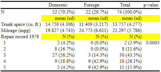
In this table, we have added some string items such as “mean(sd)” and “N(%)”, and they are highlighted in yellow.
Please note that the shading color will not be reflected in the Results window because this formatting is not available with SMCL. Style changes will be reflected in the exported file and in the Tables Builder for Windows and Mac. Please see FAQ: Why can't I observe the style changes (background shading, font, etc.) in my table in the Results window? for more detailed information.
This time, we are creating some new rows instead of new columns. I opted for two new row tags, var[newline1] and var[newline2], to identify those rows, which is straightforward. However, deciding the proper column tags is a more challenging task.
The current column tags are foreign#result result[p], and we do not need to care about result[p] because it is a separate column. Our focus is to know which exact levels are in the interaction foreign#result. We utilize collect levelsof to inspect all the levels within a specific dimension.
. collect levelsof foreign

Collection: DTable
 Dimension: foreign
    Levels: 0 1 .m
As we can see, foreign has three levels, 0, 1, and .m, which correspond to the columns of Domestic, Foreign, and Total, respectively. We will check the same information for result:
. collect levelsof result

Collection: DTable
 Dimension: result
    Levels: _dtable_stats _dtable_test frequency fvfrequency
fvpercent mean p percent proportion rawpercent rawproportion sd sumw
We notice there are a lot more levels in the dimension result. Apparently, they are not all used in the table. Let's check the automatic levels for this dimension, which are the levels that are automatically included when we only specify the dimension name in the table layout.
. collect query autolevels result

Automatic dimension levels
Collection: DTable
 Dimension: result
    Levels: _dtable_stats _dtable_test p
For more information about automatic levels of a dimension, please refer to FAQ: What are the autolevels of a dimension in a table (collection)?
We see three autolevels for the dimension result: _dtable_stats, _dtable_test, and p. But which one is used in the first three columns? _dtable_test is missing because we do not request tests in the call to dtable. And p is used only in the fourth column. So we know result[_dtable_stats] is what shows up in the first three columns. In fact, _dtable_stats is a composite result that consists of multiple results. Now let's examine the elements of this composite result.
. collect query composite _dtable_stats

Composite definition
Collection: DTable
 Composite: _dtable_stats
  Elements: frequency
            percent
            mean
            sd
            fvfrequency
            fvpercent
 Delimiter: " "
      Trim: on
  Override: off
We can see the composite result result[_dtable_stats] includes six elements, result[frequency], result[percent], result[mean], result[sd], result[fvfrequency], and result[fvpercent], which are all the statistics involved in the original descriptive table generated by dtable. Although all six statistics may not be available simultaneously on each row, any available ones will be visible. For example, on the first row result[frequency] and result[percent] are available and visible; and on the third row result[mean] and result[sd] are available. The composite result is created by the initial dtable command.
Please note that we cannot directly add new items to the collection under composite results, but we can add new items to the specific elements of this composite result, such as result[mean] or result[percent]. And the items will show up where result[_dtable_stats] defines the table layout. Proper additional tags such as var[newline1] and foreign[0] should be attached to the items, corresponding to the specific row and column we intend to place them in the final table. Here is the code we attempt to run:
collect get mean="mean (sd)", tags(foreign[0] var[newline1])
collect get mean="mean (sd)", tags(foreign[1] var[newline1])
collect get mean="mean (sd)", tags(foreign[.m] var[newline1])

collect get mean="N(%)", tags(foreign[0] var[newline2])
collect get mean="N(%)", tags(foreign[1] var[newline2])
collect get mean="N(%)", tags(foreign[.m] var[newline2])

* the autolevels of result is modified by the above commands. Let’s reset it
collect style autolevels result _dtable_stats, clear
collect style autolevels var _N newline1 trunk mpg newline2 1.rep78 2.rep78 3.rep78 4.rep78 5.rep78, clear

* hide the row header for the added rows
collect style header var[newline1 newline2] , level(hide)

collect layout (var) (foreign#result result[p])
Here is the resulting table:
| Domestic Foreign Total p-value |
| N 52 (70.3%) 22 (29.7%) 74 (100.0%) |
| mean (sd) mean (sd) mean (sd) Trunk space (cu. ft.) 14.750 (4.306) 11.409 (3.217) 13.757 (4.277) Mileage (mpg) 19.827 (4.743) 24.773 (6.611) 21.297 (5.786) N(%) N(%) N(%) Repair record 1978 1 2 (4.2%) 0 (0.0%) 2 (2.9%) 0.0005 2 8 (16.7%) 0 (0.0%) 8 (11.6%) 3 27 (56.2%) 3 (14.3%) 30 (43.5%) 4 9 (18.8%) 9 (42.9%) 18 (26.1%) 5 2 (4.2%) 9 (42.9%) 11 (15.9%) |
This is almost like what we are after, except for one thing: the content “N (%)” does not appear in the same row as “Repair record 1978”; instead, it appears in a row above it. This is because the row tag var[newline2] introduces a separate new row. This can be resolved by switching the tags for rep78 from var to rep78.
In the collection, there are two dimensions that can represent the levels of the variable rep78; one is var and another is rep78 (each categorical variable shown in this table has a corresponding dimension with the same name as the variable). In most of the cases, these two dimensions can be used interchangeably. This is because each item in the collection that has the tag var[#.rep78], should also have a tag rep78[#]. So using either of these two dimensions should produce the same results. For example, the two commands below produce similar tables:
. collect layout (var[2.rep78 3.rep78]) (foreign#result)

. collect layout (rep78[2 3]) (foreign#result)
. collect layout (var[2.rep78 3.rep78]) (foreign#result)

Collection: DTable
      Rows: var[2.rep78 3.rep78]
   Columns: foreign#result
   Table 1: 3 x 3
| Domestic Foreign Total |
| Repair record 1978 2 8 (16.7%) 0 (0.0%) 8 (11.6%) 3 27 (56.2%) 3 (14.3%) 30 (43.5%) |
. collect layout (rep78[2 3]) (foreign#result)

Collection: DTable
      Rows: rep78[2 3]
   Columns: foreign#result
   Table 1: 2 x 3
| Domestic Foreign Total |
| 2 8 (16.7%) 0 (0.0%) 8 (11.6%) 3 27 (56.2%) 3 (14.3%) 30 (43.5%) |
We can observe that the table content from the above two tables is the same, except for the difference in header style, which can be adjusted later.
But the question is why we should use rep78 instead of var for our table. This is because rep78, or any other categorical variable’s dimension, can include a _hide level, displaying content on the same row as the variable label without introducing a new row to the table. This feature will put “N (%)” in the same row as “Repair record 1978”.
Here's the final complete code, which also adds the shading color for the new table content.
clear all
sysuse auto
dtable trunk mpg i.rep78, by(foreign) column(by(hide))
logistic foreign i.rep78
testparm i.rep78
collect get r(p), tags(var[1.rep78])
collect layout (var) (foreign#result result[p])
collect label levels result p "p-value", modify
collect style header result[p], level(label)
collect style cell result[p], nformat(%21.4fc)


collect get mean="mean (sd)", tags(foreign[0] var[newline1])
collect get mean="mean (sd)", tags(foreign[1] var[newline1])
collect get mean="mean (sd)", tags(foreign[.m] var[newline1])

collect get frequency="N (%)", tags(foreign[0] rep78[_hide])
collect get frequency="N (%)", tags(foreign[1] rep78[_hide])
collect get frequency="N (%)", tags(foreign[.m] rep78[_hide])

collect style autolevels result _dtable_stats, clear
collect style autolevels var _N newline1 trunk mpg, clear
collect style autolevels rep78 _hide 1 2 3 4 5 6, clear

collect style header var[newline1], level(hide)

collect style header rep78, title(label)
collect style cell var[newline1]#cell_type[item], shading( background(yellow))
collect style cell rep78[_hide]#cell_type[item], shading( background(yellow))

collect layout (var rep78) (foreign#result result[p])
This code creates the table we want. Let's export the table to an .html file and view the resulting file.
. collect export a.html, replace
To read more, please refer to our Stata Customizable Tables and Collected Results Reference Manual.


