What is the exact time of cancer recurrence? Or time of COVID-19 infection? We don't really know exactly. All we know is that the cancer recurred sometime between two follow-up examinations and that the infection occurred sometime before the onset of symptoms or a positive COVID test. These are examples of interval-censored and left-censored time-to-event data. By time-to-event or event-time data, we also mean failure-time data, duration data, and so on.

Interval-censored event-time data arise in many areas, including medical, epidemiological, economic, financial, and sociological studies. Ignoring interval-censoring will often lead to biased estimates.

A semiparametric Cox proportional hazards regression model is used routinely to analyze uncensored and right-censored event-time data. In Stata 17, you can use the new estimation command stintcox to fit the Cox model to interval-censored event-time data.

Just as with right-censored data, a Cox model is appealing for interval-censored data because it uses semiparametric estimation and thus does not require any parametric assumptions about the baseline hazard function. Also for low-event rates, the exponentiated regression parameters approximate the log relative-risks.

Semiparametric estimation of interval-censored event-time data is challenging because none of the event times are observed exactly. Thus, "semiparametric" modeling of these data often resorted to using spline methods or piecewise-exponential models for the baseline hazard function. Genuine semiparametric modeling of interval-censored event-time data was not available until recent methodological advances, which are implemented in the stintcox command.

Let's see it work

• Estimation
• Graphing survivor functions
• Stratification
• Checking proportional-hazards assumption
• Additional resources

Estimation

We use data from Zeng, Mao, and Lin (2016), who study time to HIV infection in a cohort study of injecting drug users in Thailand. The dataset contains 1,124 subjects. Those subjects initially tested negative for the HIV virus. They were then followed and assessed for HIV-1 seropositivity through blood tests approximately every four months. Because the subjects were tested periodically, the exact time of HIV infection was not observed, but it was known to fall in intervals between blood tests with the lower and upper endpoints recorded in variables ltime and rtime.

We want to identify the factors that influence time to HIV infection. The factors we are interested in are age at recruitment (age), sex (male), history of needle sharing (needle), history of drug injection (inject), and whether a subject has been in jail at the time of recruitment (jail).

. use https://www.stata-press.com/data/r17/idu
(Bangkok Tenofovir Study (BTS))

. describe

Contains data from https://www.stata-press.com/data/r17/idu.dta
 Observations:         1,124                  Modified Bangkok IDU Preparatory
                                                Study
    Variables:             8                  15 Dec 2020 13:34
                                              (_dta has notes)


Variable      Storage   Display    Value                    
    name         type    format    label      Variable label

age             byte    %8.0g                 Age (in years)
male            byte    %8.0g      yesno      Male
needle          byte    %8.0g      yesno      Shared needles
jail            byte    %8.0g      yesno      Imprisoned
inject          byte    %8.0g      yesno      Injected drugs before recruitment
ltime           double  %10.0g                Last time seronegative for HIV-1
rtime           double  %10.0g                First time seropositive for HIV-1
age_mean        double  %10.0g                Centered age (in years)

We fit a Cox proportional hazards model in which time to HIV infection depends on the above factors of interest. To make the interpretation of the baseline hazard function more reasonable, we will use the centered age variable, age_mean.

. stintcox age_mean i.male i.needle i.inject i.jail, interval(ltime rtime)
note: using adaptive step size to compute derivatives.

Performing EM optimization (showing every 100 iterations):
Iteration 0:    log likelihood = -1086.2564
Iteration 100:  log likelihood = -597.65634
Iteration 200:  log likelihood = -597.57555
Iteration 295:  log likelihood = -597.56443

Computing standard errors: ............................ done

Interval-censored Cox regression                    Number of obs     =  1,124
Baseline hazard: Reduced intervals                         Uncensored =      0
                                                        Left-censored =     41
                                                       Right-censored =    991
                                                       Interval-cens. =     92

                                                    Wald chi2(5)      =  17.10
Log likelihood = -597.56443                         Prob > chi2       = 0.0043


             
 
                 OPG
             
 
 Haz. ratio   std. err.      z    P>|z|     [95% conf. interval]

    age_mean 
 
   .9684341   .0126552    -2.45   0.014     .9439452    .9935582
 

        male 
 

        Yes  
 
   .6846949   .1855907    -1.40   0.162     .4025073    1.164717
 

      needle 
 

        Yes  
 
   1.275912   .2279038     1.36   0.173     .8990401    1.810768
 

      inject 
 

        Yes  
 
   1.250154   .2414221     1.16   0.248     .8562184    1.825334
 

        jail 
 

        Yes  
 
   1.567244   .3473972     2.03   0.043     1.014982    2.419998

Note: Standard-error estimates may be more variable for small datasets and
      datasets with low proportions of interval-censored observations.

We find that age at recruitment is associated with lower risk of HIV infection and being in jail at enrollment is associated with higher risk of HIV infection. Other factors are not statistically significant.

Graphing survivor functions

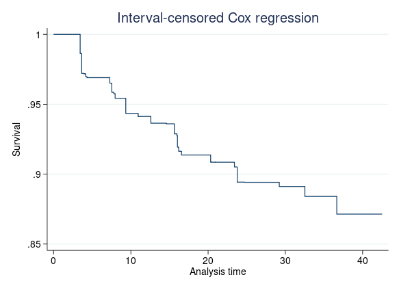
We can graph the baseline survival curve by using stcurve with all covariates set to 0.

. stcurve, survival at((zero) _all)

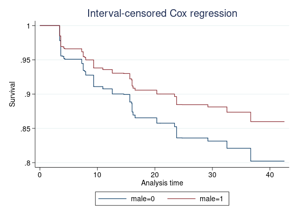
We can also graph the survivor functions with covariates set to any value. Suppose we want to compare the survivor functions of an average subject in the female and male groups. We type

. stcurve, survival at(male=(0 1))

Stratification

If we assume that the baseline hazard function for female is different from that for male, we can fit a stratified Cox proportional hazards model by using the strata() option:

. stintcox age_mean i.needle i.inject i.jail, interval(ltime rtime) strata(male)
note: using adaptive step size to compute derivatives.

Performing EM optimization (showing every 100 iterations):
Iteration 0:    log likelihood = -1087.0536
Iteration 100:  log likelihood = -585.59848
Iteration 200:  log likelihood = -585.53143
Iteration 282:  log likelihood =  -585.5222

Computing standard errors: ........................... done

Stratified interval-censored Cox regression
Baseline hazard: Reduced intervals

Strata variable: male                               Number of obs     =  1,124
                                                           Uncensored =      0
                                                        Left-censored =     41
                                                       Right-censored =    991
                                                       Interval-cens. =     92

                                                    Wald chi2(4)      =  14.84
Log likelihood = -585.5222                          Prob > chi2       = 0.0051


             
 
                 OPG
             
 
 Haz. ratio   std. err.      z    P>|z|     [95% conf. interval]

    age_mean 
 
   .9682508   .0126326    -2.47   0.013     .9438052    .9933295
 

        male 
 

        Yes  
 
   1.276222   .2270302     1.37   0.170     .9005422    1.808625
 

      needle 
 

        Yes  
 
   1.245357   .2393768     1.14   0.254     .8544367    1.815131
 

      inject 
 

        Yes  
 
   1.245357   .2393768     1.14   0.254     .8544367    1.815131
 

        jail 
 

        Yes  
 
    1.57314   .3490687     2.04   0.041     1.018337    2.430205

Note: Standard-error estimates may be more variable for small datasets and
      datasets with low proportions of interval-censored observations.

Our conclusion here is similar to the case without stratification.

Checking proportional-hazards assumption

It is important to evaluate the validity of the underlying assumption for the Cox proportional hazards model, which is that the hazard ratio is constant over time. Stata 17 provides two new graphical commands to assess the proportional-hazards assumption.

For a single categorical covariate in a Cox model, you can use stintphplot, which plots -ln{-ln(survival)} curves for each category versus ln(analysis time). If the plots are parallel, the proportional-hazards assumption has not been violated. Alternatively, you can use stintcoxnp to plot the nonparametric maximum-likelihood estimation survival curve versus the Cox predicted survival curve for each category. When the two curves are close together, the proportional-hazards assumption is valid.

When a Cox model contains multiple covariates, as mentioned in the above example, only stintphplot is appropriate for testing the proportional-hazards assumption. In that case, we need to use the adjustfor() option.

For example, to check the proportional-hazards assumption for inject, we include all covariates except inject in the adjustfor() option:

. stintphplot, interval(ltime rtime) by(inject) adjustfor(age_mean i.male i.needle i.jail)

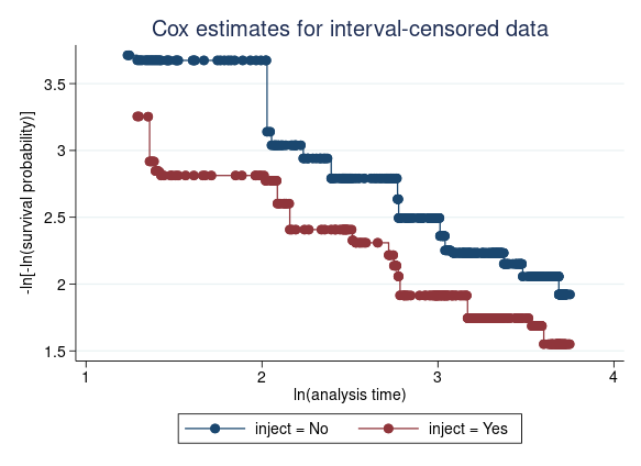
A separate Cox model, which contains all covariates from the adjustfor() option, is fit for each level of inject. And the two plots are almost parallel, which indicates that the proportional-hazards assumption has not been violated for the categorical variable inject.

Reference

Zeng, D., L. Mao, and D. Lin. 2016. Maximum likelihood estimation for semiparametric transformation models with interval-censored data. Biometrika 103: 253–271.

Additional resources

Learn more in [ST] stintcox.

Learn more about parametric interval-censored event-time models.

View all the new features