
1 item has been added to your cart.
Mixed logit models are models for choice outcomes. Choices might be modes of transportation, car insurance providers, or types of vacations.
Sometimes individuals make the same decision repeatedly:
When data contain repeated choices, we have panel data.
With Stata 16's new cmxtmixlogit command, you can fit panel-data mixed logit models.
Like other choice models, mixed logits model the probability of selecting alternatives based on a group of covariates. Mixed logit models are special in that they use random coefficients to model the correlation of choices across alternatives. These random coefficients allow us to relax the independence of the irrelevant alternatives (IIA) assumption that is required by some other choice models. IIA says that if you have a choice of walking, riding a bike, or driving a car, and you choose walking, then once you have made your choice, the other alternatives should be irrelevant. If we took away one of the other alternatives, you would still choose walking, right? Maybe not. Human beings sometimes violate the IIA assumption.
In the context of panel-data applications, we can use mixed logit models to model the probability of selecting each alternative for each time period rather than modeling a single probability for selecting each alternative, as in the case of cross-sectional data.
Stata can fit many other choice models. And the entire suite of choice model commands has been improved and expanded. You can read all about that here.
We want to learn about the effects of travel cost on the choice of transportation mode to the workplace. In particular, we would like to know the following:
We can use the cmxtmixlogit command followed by margins to answer these questions and more.
Let's take a look at a portion of our panel data:
. list id t alt choice in 1/12, sepby(t) noobs
| id t alt choice |
| 1 1 Car 1 |
| 1 1 Public 0 |
| 1 1 Bicycle 0 |
| 1 1 Walk 0 |
| 1 2 Car 1 |
| 1 2 Public 0 |
| 1 2 Bicycle 0 |
| 1 2 Walk 0 |
| 1 3 Car 1 |
| 1 3 Public 0 |
| 1 3 Bicycle 0 |
| 1 3 Walk 0 |
Each individual has an ID code stored in the variable id, and t contains the time period at which a decision was made. Here we have three time periods for individual 1. The alternatives are recorded in the variable alt. The variable choice records the chosen alternative. This individual drove a car to work in all three time periods.
Our data also include information on the travel, the cost, the individual's age, and his or her income. Both travel time and cost are alternative specific–they vary across alternatives. Age and income are case specific–they are constant within a single time period for each individual.
Before we fit our panel-data mixed logit model, we use cmset to tell Stata about the variables in our data that identify individuals, time periods, and alternatives.
. cmset id t alt
panel data: panels id and time t
note: case identifier _caseid generated from id t
note: panel by alternatives identifier _panelaltid generated from id alt

                     caseid variable:  _caseid
               alternatives variable:  alt
      panel by alternatives variable:  _panelaltid (strongly balanced)
                       time variable:  t, 1 to 3
                               delta:  1 unit

note: data have been xtset
We can now use cmxtmixlogit to fit our model.
We wish to estimate the effect of travel cost (trcost) on the choice of transportation mode, controlling for travel time, income, and age. We assume that all individuals have the same preferences with respect to travel cost. But we assume that preferences with respect to travel time are heterogeneous, and we model these heterogeneous preferences with a random coefficients for trtime.
We specify that choice contains the chosen alternatives and that trcost is included in the model with a fixed coefficient. The option random(trtime) includes trtime in the model with a normally distributed random coefficient (the default distribution for random coefficients). Because age and income are case specific, we include them using the casevars() option and estimate a fixed coefficient for each one.
. cmxtmixlogit choice trcost, random(trtime) casevars(age income) nolog

Mixed logit choice model                     Number of obs        =      6,000
                                             Number of cases      =      1,500
Panel variable: id                           Number of panels     =        500

Time variable: t                             Cases per panel: min =          3
                                                              avg =        3.0
                                                              max =          3

Alternatives variable: alt                   Alts per case:   min =          4
                                                              avg =        4.0
                                                              max =          4
Integration sequence:      Hammersley
Integration points:               594             Wald chi2(8)    =     432.68
Log simulated likelihood = -1005.9899             Prob > chi2     =     0.0000
| choice | Coef. Std. Err. z P>|z| [95% Conf. Interval] | |
| alt | ||
| trcost | -.8388216 .0438587 -19.13 0.000 -.9247829 -.7528602 | |
| trtime | -1.508756 .2641554 -5.71 0.000 -2.026492 -.9910212 | |
| /Normal | ||
| sd(trtime) | 1.945596 .2594145 1.498161 2.526661 | |
| Car | (base alternative) | |
| Public | ||
| age | .1538915 .0672638 2.29 0.022 .0220569 .2857261 | |
| income | -.3815444 .0347459 -10.98 0.000 -.4496451 -.3134437 | |
| _cons | -.5756547 .3515763 -1.64 0.102 -1.264732 .1134222 | |
| Bicycle | ||
| age | .20638 .0847655 2.43 0.015 .0402426 .3725174 | |
| income | -.5225054 .0463235 -11.28 0.000 -.6132978 -.4317131 | |
| _cons | -1.137393 .4461318 -2.55 0.011 -2.011795 -.2629909 | |
| Walk | ||
| age | .3097417 .1069941 2.89 0.004 .1000372 .5194463 | |
| income | -.9016697 .0686042 -13.14 0.000 -1.036132 -.7672078 | |
| _cons | -.4183279 .5607112 -0.75 0.456 -1.517302 .6806458 | |
The estimate of the fixed coefficient on trcost is -0.84. The estimated mean of the random coefficients on trtime is -1.51 with an estimated standard deviation of 1.95, indicating considerable heterogeneity in these coefficients over the individuals in the population.
What can we learn from these results? We can say that if travel cost increases for a certain alternative, the chance of choosing that alternative decreases. In other words, people do not like to waste money–something that we may not consider a groundbreaking discovery. Remember that what we really wanted to know was how the probability of choosing a certain alternative changes if we change travel cost related to that alternative and how that affects the probability of choosing any of the other alternatives. Using just the above model results, we have no answer to these questions. We can, however, find an answer to these questions by using margins:
. margins, outcome(Car) alternative(Car)
           at(trcost = generate(trcost))
           at(trcost = generate(1.25*trcost))
           over(t)

Predictive margins                              Number of obs     =      6,000
Model VCE    : OIM

Expression   : Pr(alt), predict()
Alternative  : Car
Outcome      : Car
over         : t

1._at        : 1.t
                   trcost          = trcost
               2.t
                   trcost          = trcost
               3.t
                   trcost          = trcost

2._at        : 1.t
                   trcost          = 1.25*trcost
               2.t
                   trcost          = 1.25*trcost
               3.t
                   trcost          = 1.25*trcost
| Delta-method | ||
| Margin Std. Err. z P>|z| [95% Conf. Interval] | ||
| _at#t | ||
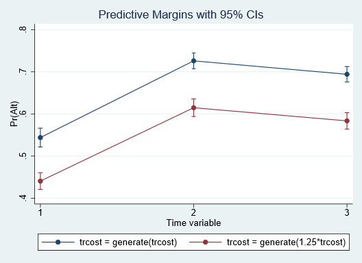
| 1 1 | .5439062 .0113994 47.71 0.000 .5215638 .5662486 | |
| 1 2 | .7259769 .0095234 76.23 0.000 .7073114 .7446425 | |
| 1 3 | .6940885 .0093699 74.08 0.000 .6757238 .7124532 | |
| 2 1 | .4405694 .0101017 43.61 0.000 .4207704 .4603683 | |
| 2 2 | .6147295 .0106749 57.59 0.000 .5938071 .6356518 | |
| 2 3 | .583544 .0099536 58.63 0.000 .5640354 .6030527 | |
Here we estimate expected probabilities of choosing each outcome under two scenarios, labeled _at. The first scenario is the as is scenario: all variables are as observed. In the second scenario, the cost of car travel increases by 25%. We do this by specifying the option alternative(Car) to tell margins that we wish to apply our at() scenarios for the alternative-specific variable trcost to the car alternative. And we specify outcome(Car) to tell margins that we wish to estimate the averaged probabilities of choosing the car alternative. We specify over(t) to compute the averaged probabilities for each time period.
Looking at the first time period, we expect the individuals in our population to choose to drive a car with a probability of 0.54 with car travel cost as is. And if we increase car travel cost by 25%, the probability of choosing the car decreases by around 0.1 to 0.44. We can visualize the expected probabilities over all time periods by using marginsplot.
Because we are actually interested in the differences between the two scenarios, we can compute these directly using the contrast() option:
. margins, outcome(Car) alternative(Car)
           at(trcost = generate(trcost))
           at(trcost = generate(1.25*trcost))
           over(t) contrast(at(r) nowald)

Contrasts of predictive margins                 Number of obs     =      6,000
Model VCE    : OIM

Expression   : Pr(alt), predict()
Alternative  : Car
Outcome      : Car
over         : t

1._at        : 1.t
                   trcost          = trcost
               2.t
                   trcost          = trcost
               3.t
                   trcost          = trcost

2._at        : 1.t
                   trcost          = 1.25*trcost
               2.t
                   trcost          = 1.25*trcost
               3.t
                   trcost          = 1.25*trcost
| Delta-method | ||
| Contrast Std. Err. [95% Conf. Interval] | ||
| _at@t | ||
| (2 vs 1) 1 | -.1033369 .0025876 -.1084084 -.0982653 | |
| (2 vs 1) 2 | -.1112475 .0034421 -.1179938 -.1045011 | |
| (2 vs 1) 3 | -.1105445 .0028249 -.1160812 -.1050078 | |
The differences in expected probabilities are similar across time periods, ranging from -0.10 to -0.11 when comparing the original price with the 25% increase.
To answer our second question–how does change in price of car travel affect the probability of public transportation–we simply specify outcome(Public) instead of outcome(Car).
. margins, outcome(Public) alternative(Car)
           at(trcost = generate(trcost))
           at(trcost = generate(1.25*trcost))
           over(t) contrast(at(r) nowald)

Contrasts of predictive margins                 Number of obs     =      6,000
Model VCE    : OIM

Expression   : Pr(alt), predict()
Alternative  : Car
Outcome      : Public
over         : t

1._at        : 1.t
                   trcost          = trcost
               2.t
                   trcost          = trcost
               3.t
                   trcost          = trcost

2._at        : 1.t
                   trcost          = 1.25*trcost
               2.t
                   trcost          = 1.25*trcost
               3.t
                   trcost          = 1.25*trcost
| Delta-method | Contrast Std. Err. [95% Conf. Interval] | |
| _at@t | ||
| (2 vs 1) 1 | .0538434 .0022563 .0494212 .0582656 | (2 vs 1) 2 | .0683515 .0032234 .0620338 .0746692 | (2 vs 1) 3 | .0671689 .0029154 .0614547 .072883 |
We find that the expected probability of using public transportation goes up by 0.05, or 5 percentage points, in the first time period if car travel costs increase by 25%.
margins allows one to answer many other interesting questions after panel-data mixed logit models. We show additional examples of using margins after choice models here. Everything we do there can be done after cmxtmixlogit. And there's much more.
Learn more about Stata's choice model features.
Learn more about Stata's commands for choice models in the Stata Choice Model Reference manual.
For more information about cmxtmixlogit, see [CM] cmxtmixlogit.
For more about inference using margins, see [CM] Intro 1.


