Ordinal variables are categorical and ordered, such as poor, fair, good, very good, and excellent. One way to think about ordered variables is that the categories represent ranges of an unobserved continuous variable z. The mapping might be

poor                z ≤ -1.72
fair        -1.72 < z ≤ -0.93
good        -0.93 < z ≤ -0.02
very good   -0.02 < z ≤  0.89
excellent    0.89 < z

Perhaps the categories are for overall health.

If z were distributed normal with mean 0 and standard deviation 1, the above would be an ordered probit model. It would correspond to 4% of subjects reporting poor, 13% reporting fair, and so on.

Stata would fit this model if you used its ordered probit command oprobit and typed

. oprobit health

You could instead specify a linear function for z in terms of age, bmi, and i.exercise by typing

. oprobit health age bmi i.exercise

The fitted model might be

z = -0.0083*age - 0.0469*bmi + 0.5596*i.exercise

and the corresponding mapping be

poor                z ≤ -3.30
fair        -3.30 < z ≤ -2.39
good        -2.39 < z ≤ -1.39
very good   -1.39 < z ≤ -0.38
excellent    0.89 < z

It would, however, be reasonable to assume that health status varies more as age increases; Stata's new hetoprobit command can handle that. You would type

. hetoprobit health age bmi i.exercise, het(age)

Let's see it work

We have data from the 2015 Eating & Health Module of the American Time Use Survey (ATUS) of the U.S. Bureau of Labor Statistics. If we type the above command with these data, the result is

. hetoprobit health age bmi i.exercise, het(age)

Fitting cutpoints-only heteroskedastic model:

Iteration 0:   log likelihood = -2905.7943
Iteration 1:   log likelihood = -2898.4819
Iteration 2:   log likelihood = -2897.9184
Iteration 3:   log likelihood = -2897.9167
Iteration 4:   log likelihood = -2897.9167

Fitting ordered probit model:

Iteration 0:   log likelihood = -2905.7943
Iteration 1:   log likelihood = -2717.2752
Iteration 2:   log likelihood = -2716.9679
Iteration 3:   log likelihood = -2716.9679

Fitting full model:

Iteration 0:   log likelihood = -2716.9679
Iteration 1:   log likelihood = -2710.6282
Iteration 2:   log likelihood = -2710.2321
Iteration 3:   log likelihood =  -2710.231
Iteration 4:   log likelihood =  -2710.231

Heteroskedastic ordered probit regression       Number of obs     =      2,009
                                                LR chi2(3)        =     375.37
Log likelihood =  -2710.231                     Prob > chi2       =     0.0000



      health 
 
      Coef.   Std. Err.      z    P>|z|     [95% Conf. Interval]

health       
 
                                                               
         age 
 
 -.0088414   .0016631    -5.32   0.000     -.012101   -.0055817
         bmi 
 
 -.0585007   .0058617    -9.98   0.000    -.0699893    -.047012
             
 
                                                               
    exercise 
 
                                                               
         yes 
 
  .6892342   .0729718     9.45   0.000      .546212    .8322563

lnsigma      
 
                                                               
         age 
 
  .0042449   .0011597     3.66   0.000     .0019719    .0065179

       /cut1 
 
 -4.063604   .2892444                     -4.630512   -3.496695
       /cut2 
 
 -2.902873   .2249795                     -3.343825   -2.461922
       /cut3 
 
 -1.645604   .1777954                     -1.994077   -1.297132
       /cut4 
 
 -.4148757     .15937                     -.7272352   -.1025162


LR test of lnsigma=0: chi2(1) = 13.47                     Prob > chi2 = 0.0002

The result is

z = -0.0088*age - 0.0585*bmi + 0.6892*i.exercise

with corresponding mapping

poor                z ≤ -4.06
fair        -4.06 < z ≤ -2.90
good        -2.90 < z ≤ -1.65
very good   -1.65 < z ≤ -0.41
excellent   -0.41 < z

These results account for the possible increased variation (heteroskedasticity) due to age.

Is there such heteroskedasticity? There is according to the output chi2(1) = 13.47.

Does it make a difference? Let's compare coefficients with those we previously calculated using oprobit:

z = -0.0083*age - 0.0469*bmi + 0.5596*i.exercise  (orig.)
z = -0.0088*age - 0.0585*bmi + 0.6892*i.exercise  (adj)

The effect of i.exercise has changed, although perhaps not significantly.

Here is a graph of the predicted probability of very good or excellent health against body mass index.

. predict pr*                      // predicted Pr(each outcome)
(option pr assumed; predicted probabilities)
(107 missing values generated)

. generate pr45 = pr4 + pr5        // Pr(very good or better)
(107 missing values generated)

. graph twoway scatter pr45 bmi,
  ytitle("Pr(very good or better health)") 
  title("Effect of BMI on predicted probability")

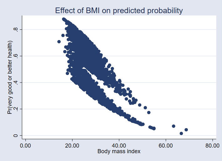
Does the division into distinct groups surprise you? It did us. It turns out that the top group exercises and the lower group does not.

Tell me more

Read more about heteroskedastic ordered probit models in the Stata Base Reference Manual; see [R] hetoprobit.