1 item has been added to your cart.
Nonparametric regression, like linear regression, estimates mean outcomes for a given set of covariates. Unlike linear regression, nonparametric regression is agnostic about the functional form between the outcome and the covariates and is therefore not subject to misspecification error.
In nonparametric regression, you do not specify the functional form. You specify the dependent variable—the outcome—and the covariates. You specify \(y, x_1, x_2,\) and \(x_3\) to fit
\[ y = g(x_1, x_2, x_3) + \epsilon \]
The method does not assume that \(g( )\) is linear; it could just as well be
\[ y = \beta_1 x_1 + \beta_2 x_2^2 + \beta_3 x_1^3 x_2 + \beta_4 x_3 + \epsilon \]
The method does not even assume the function is linear in the parameters. It could just as well be
\[ y = \beta_1 x_1^{\beta_2} + cos(x_2 x_3) + \epsilon \]
Or it could be anything else.
The result is not returned to you in algebraic form, but predicted values and derivatives can be calculated. To fit whatever the model is, you type
. npregress kernel y x1 x2 x3
npregress needs more observations than linear regression to produce consistent estimates, of course, but perhaps not as many extra observations as you would expect. A model like this one could easily be fit on 500 observations.
We have fictional data on wine yield (hectoliters) from 512 wine-producing counties around the world. That will be our dependent variable. We believe output is affected by
| taxlevel | taxes on wine production |
| rainfall | rainfall in mm/hour |
| avgtemp | average temperature in degrees Celsius |
| irrigate | whether winery irrigates |
| organic | whether winery uses organic fertilizers |
We will ultimately fit a model of hectoliters on all the above variables, but we will start with a model of hectoliters on taxlevel so that we can show you a graph of the result, which is the nonlinear function that npregress produces.
First, we fit the model:
. npregress kernel hectoliters taxlevel, vce(bootstrap, reps(100) seed(123))
(running npregress on estimation sample)

Bootstrap replications (100)
----+--- 1 ---+--- 2 ---+--- 3 ---+--- 4 ---+--- 5
..................................................    50
..................................................   100

Bandwidth
| Mean Effect | ||
| Mean | ||
| taxlevel | .0116542 .0175038 | |
| Observed Bootstrap Percentile | ||
| hectoliters | Estimate Std. Err. z P|>z| [95% Conf. Interval] | |
| Mean | ||
| hectoliters | 432.5049 .8204567 527.15 0.000 431.2137 434.1426 | |
| Effect | ||
| taxlevel | -312.0013 15.78939 -19.76 0.000 -345.4684 -288.3484 | |
There are two parts to the output. The first part reports two bandwidths, one for calculating the mean and the other for calculating the effect. These are technical details but sometimes useful.
The second part reports the fitted results as a summary about the fitted model's predictions. The first summary is about the average predicted value of hectoliters given taxlevel and is not especially interesting. It is 433. The second summary is more interesting. It reports the average derivative of hectoliters with regard to taxlevel, what economists would call the marginal effect of taxes on production. It is −312. That means higher taxes result in lower output. It is significant, too.
At this point, you may be thinking you could have obtained a different kind of average tax effect using linear regression. You would be right. You could have typed regress hectoliters taxlevel, and you would have obtained −245 as the average effect.
npregress provides more information than just the average effect. It fit an entire functon and we can graph it. The function is shown in red on top of the data:
. npgraph
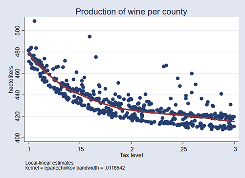
The effect of taxes is not linear! In fact, you now understand why regress reported a smaller average effect than npregress reported. The tax-level effect is bigger on the front end.
We wanted you to see the nonlinear function before we fit a model in higher dimensional space. In higher dimensional space, we will not be able to graph the function using npgraph, but we will be able to use Stata's margins and marginsplot commands to obtain and help us visualize the effects.
Here is our full model:
. npregress kernel hectoliters taxlevel rainfall avgtemp i.organic
           i.irrigate, vce(bootstrap, reps(100) seed(123))
(running npregress on estimation sample)

Bootstrap replications (100)
----+--- 1 ---+--- 2 ---+--- 3 ---+--- 4 ---+--- 5
..................................................    50
..................................................   100

Bandwidth
| Mean Effect | ||
| Mean | ||
| taxlevel | .0143197 .0200742 | |
| rainfall | .0667891 .0936294 | |
| avgtemp | 2.997119 4.201559 | |
| organic | .5019867 .5019867 | |
| irrigate | .5225674 .5225674 | |
| Observed Bootstrap Percentile | ||
| hectoliters | Estimate Std. Err. z P>|z| [95% Conf. Interval] | |
| Mean | ||
| hectoliters | 433.2502 .8344479 519.21 0.000 431.6659 434.6313 | |
| Effect | ||
| taxlevel | -291.8007 11.71411 -24.91 0.000 -318.3464 -271.3716 | |
| rainfall | 62.60715 4.626412 13.53 0.000 53.16254 71.17432 | |
| avgtemp | .0346941 .0261008 1.33 0.184 -.0069348 .0956924 | |
| organic | ||
| (1 vs 0) | 7.09874 .3207509 22.13 0.000 6.527237 7.728458 | |
| irrigate | ||
| (1 vs 0) | 6.967769 .3056074 22.80 0.000 6.278343 7.533998 | |
Reported are average effects for each of the covariates.
To help us understand the function, we can use margins. What would happen to output if tax rates were increased by 15%? The answer is that output would fall by 36.9 hectoliters, or about 8.5%:
. margins, at(taxlevel=generate(taxlevel))
           at(taxlevel=generate(taxlevel*1.15))
           contrast(atcontrast(r) nowald)
           vce(bootstrap, reps(100) seed(123))

(running margins on estimation sample)

Bootstrap replications (100)
----+--- 1 ---+--- 2 ---+--- 3 ---+--- 4 ---+--- 5
..................................................    50
..................................................   100

Contrasts of predictive margins

                                                Number of obs     =        512
                                                Replications      =        100

Expression   : mean function, predict()

1._at        : taxlevel        = taxlevel

2._at        : taxlevel        = taxlevel*1.15
| Observed Bootstrap Percentile | ||
| Estimate Std. Err. [95% Conf. Interval] | ||
| _at | ||
| (2 vs 1) | -36.88793 4.18827 -45.37871 -29.67079 | |
We said output falls by about 8.5%. We calculated that by hand based on the −36.9 hectoliter decrease and average level of output of 432.
We can explore tax-level changes graphically, too. The above output was for a taxlevel increase of 15%. Here are the results for tax-levels of 10–30%:
. margins, at(taxlevel=(.1(.01).3))
  (output omitted)

. marginsplot
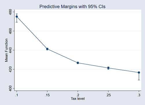
Just as in the one-variable case, we see that tax-level effects are largest at the front end.
Learn more about Stata's nonparametric methods features.
Read more about nonparametric kernel regression in the Stata Base Reference Manual; see [R] npregress intro and [R] npregress.