1 item has been added to your cart.

Power analysis for survival studies

Stata’s new stpower command provides sample-size and power calculations for survival studies that use Cox proportional-hazards regressions, log-rank tests for two groups, or parametric tests of disparity in two exponential survivor functions.

stpower cox

stpower logrank

stpower exponential

Stata’s new

1. stpower cox estimates required sample size (given power and effect size) or power (given sample size and effect size) or the minimal detectable effect size (given power and sample size) for models with multiple covariates.
2. stpower logrank estimates required sample size (given power and effect size) or power (given sample size and effect size) or the minimal detectable effect size (given power and sample size) for studies comparing survivor functions of two groups by using the log-rank test. Both the Freedman (1982) and the Schoenfeld (1981) methods are provided.
3. stpower exponential estimates sample size (given power and effect size) or power (given sample size and effect size) for parametric tests of the difference between hazards or log hazards of two groups under the assumption of exponential survivor functions. Both the Lachin and Foulkes (1986) and Rubinstein, Gail, and Santner (1981) methods are provided.

The stpower commands allow automated production of customizable tables and have options to assist with creating graphs of power curves.

Below are several examples demonstrating some of stpower’s capabilities:

• Tabulating results
• Producing power curves
• Producing customized tables

For an overview of all capabilities, see [ST] stpower.

Tabulating results

Study design
Consider a survival study comparing two treatments, a standard treatment and a new, experimental treatment. The survival probability in the control group at the end of the study is expected to be approximately 0.7. We need to estimate the sample size required to detect an increase in survival of the experimental group from 0.7 to 0.8 at the end of the study with power of 80%, 85%, and 90%, using a two-sided log-rank test at the 5% significance level. We use stpower logrank to obtain the required sample sizes:

. stpower logrank 0.7 0.8, power(0.8 0.85 0.9)

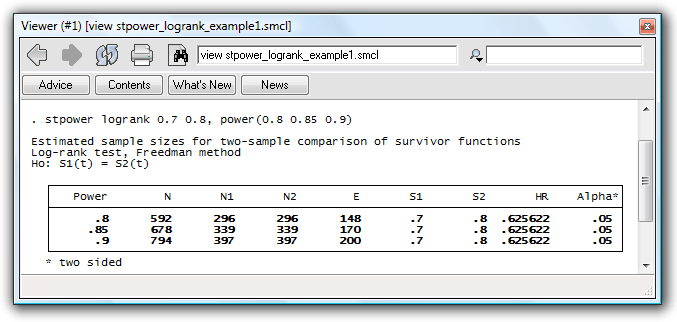
Results
The table reports estimates of the required number of events and sample sizes in the study for three powers given other study parameters. The last row of the table indicates that we need 200 events to be observed in the study (and a sample size of 794 to observe the 200 events in the study) for our log-rank test to have a power of 90%. The increase in survival from 0.7 to 0.8 is equivalent to a hazard ratio of .626 of the experimental to the control group, as shown in the second-to-last column in the table.

Producing power curves

If our sample size is predetermined, we may want to find out the smallest effect size or increase in survival expressed as a hazard ratio that can be detected with a given level of power. We can use stpower to produce power curves as a function of the hazard ratio for several sample sizes.

Suppose that we want to produce power curves as a function of the effect size for sample sizes of 100, 250, and 500 for the study we considered in the first example.

. stpower logrank 0.7, n(100 250 500) hratio(0.1(0.01)0.9) saving(mypower)

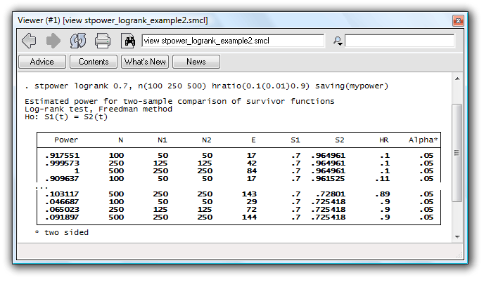
Powers are computed for each combination of sample-size and hazard-ratio values.

Producing customized tables

stpower also allows you to build your own customized tables. You can choose what to display in a table from a list of results available.

For example, if you prefer to see the probability of a type II error rather than power, and the proportion of subjects in the control group rather than group-sample sizes, reported by default, you can type

. stpower logrank 0.7 0.8, power(0.8 0.85 0.9) columns(beta n e p1 hr s1 s2 alpha)

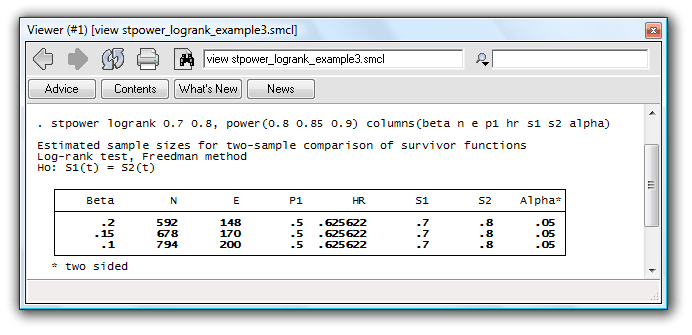
to obtain the table with requested columns displayed in the same order you specified.

Of course, all the above can be done using dialog boxes instead of the command line.

For a complete list of what’s new in survival statistics, click here.

References

Freedman, L. S. 1982.

Tables of the number of patients required in clinical trials using the logrank test. Statistics in Medicine 1: 121–129.

Lachin, J. M., and M. A. Foulkes. 1986.

Evaluation of sample size and power for analysis of survival with allowance for nonuniform patient entry, losses to follow-up, noncompliance, and stratification. Biometrics 42: 507–519.

Rubinstein, L. V., M. H. Gail, and T. J. Santner. 1981.

Planning the duration of a comparative clinical trial with loss to follow-up and a period of continued observation. Journal of Chronic Diseases 34: 469–479.

Schoenfeld, D. 1981.

The asymptotic properties of nonparametric tests for comparing survival distributions. Biometrika 68: 316–319.

Back to highlights