

StataNow spotlight: Psycho for meta-analysis
Meta-analysis quantitatively summarizes a collection of studies that address the same research question. Psychometric meta-analysis additionally corrects for statistical artifacts such as measurement error, range restriction, artificial dichotomization, and small-study bias (Schmidt and Hunter 2015). These are all common artifacts that we encounter when conducting meta-analyses in psychology and other behavioral sciences.
Why is correcting for these artifacts necessary? Let's illustrate with an experiment.
The impact of statistical artifacts
We first simulate 1,000 observations from 3 variables—x, y, and z—with the following covariance matrix:
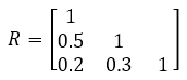
. clear

. set obs 1000
Number of observations (_N) was 0, now 1,000.

. matrix input R = (1,.5,.2\.5,1,.3\.2,.3,1)

. drawnorm x y z, corr(R) seed(12345)
Our interest lies in the relationship between x and y, which we evaluate using a Pearson correlation coefficient.
. correlate x y
(obs=1,000)
| x y | ||
| x | 1.0000 | |
| y | 0.4938 1.0000 |
We see that the observed correlation between x and y is \(r=0.494\), which is very close to their true correlation, \(ρ=0.50\).
Measurement error
Measurement error will occur anytime a scale or assessment score is of interest. Most papers will report the reliability coefficient of their measures; this is the information you would use to correct for measurement error. When it is not reported, you can impute this information or obtain it from other sources, such as psychometric papers.
What would happen if we add measurement error to x? This error variance has no association with y.
. generate x_me = x+rnormal(0,.5)

. correlate x_me y
(obs=1,000)
| x_me y | ||
| x_me | 1.0000 | |
| y | 0.4304 1.0000 |
The new variable, x_me, is x with additional random error added in. The correlation with y has decreased; it is now only \(r=0.430\).
We can also add measurement error to y.
. generate y_me = y+rnormal(0,.5)

. correlate x_me y_me
(obs=1,000)
| x_me y_me | ||
| x_me | 1.0000 | |
| y_me | 0.3849 1.0000 |
The correlation is even lower: \(r=0.385\).
This illustrates attenuation; measurement error weakens observed correlations.
Range restriction
Range restriction is common in the industrial or organizational sciences, for example, when examining only the subset of applicants who were hired or accepted into a program.
Range can be restricted either directly or indirectly.
In direct range restriction, we examine only a subset of the variables involved.
. correlate x y if x<1
(obs=840)
| x y | ||
| x | 1.0000 | |
| y | 0.3745 1.0000 |
When we examine the values of x and y only if x is less than 1, the correlation between x and y drops to \(r=0.375\).
In indirect range restriction, we restrict based on a third variable that is correlated with one or both of the variables involved.
. correlate x y if z<1
(obs=840)
| x y | ||
| x | 1.0000 | |
| y | 0.4835 1.0000 |
When we examine the values of x and y only if z is less than 1, the correlation slightly drops to \(r=0.484\). Although the attenuation is less severe in this example, you can imagine that this type of range restriction is more difficult to account for.
Artificial dichotomization
Artificial dichotomization is ubiquitous across all behavioral sciences, in which any continuous variable is dichotomized to compare two halves or create pass/fail categories, for example.
. egen x_dich = cut(x), group(2)
The new variable, x_dich, is a binary variable in which the bottom half of the observations in x were assigned 0 and the top half were assigned 1. Let’s see how this impacts its correlation with y.
. correlate x_dich y
(obs=1,000)
| x_dich y | ||
| x_dich | 1.0000 | |
| y | 0.3852 1.0000 |
We see a drastic change in the correlation coefficient to \(r=0.385\).
Small-study bias
When we conduct meta-analyses of correlations, studies with sample sizes that are less than 20 report downwardly biased correlation coefficients on average (Schmidt, Le, and Oh 2019, 320). This is known as small-study bias and is another artifact we can correct for with psychometric meta-analysis.
Now that we have seen how artifacts distort correlations, let’s analyze real data using StataNow’s meta psycorr command.
Illustrative example
Using a subset of the study information provided in Slemp et al. (2024), we examine the relationship between relatedness support and relatedness satisfaction.
We first load and describe the dataset.
. use https://www.stata.com/exdata/metaslemp.dta
(Slemp et al., 2024)

. describe

Contains data from metaslemp.dta
 Observations:            46                  Slemp et al., 2024
    Variables:             7                  1 Apr 2026 15:18
                                              (_dta has notes)
| Variable Storage Display Value | ||
| name type format label Variable label | ||
| Authors str1549 %1549s Authors N int %10.0g Study sample size age double %10.0g Mean age of sample prov long %8.0g prov Provision of relatedness support rxx double %10.0g Relatedness support reliability coefficient r double %10.0g Correlation coefficient ryy double %10.0g Relatedness satisfaction reliability coefficient | ||
We have information from 46 studies that report their sample size (N), mean age of sample (age), how relatedness support was provided (prov), the correlation between relatedness support and relatedness satisfaction (r), and the reliability coefficients of each measure (rxx and ryy, respectively).
We declare our data as psychometric meta-analysis data using the reported correlations, sample sizes, and reliabilities of each measure, and we label each study using the Authors study label. The meta psycorr command both corrects correlations for statistical artifacts and declares the data for meta-analysis, allowing seamless use of Stata’s meta-analysis tools.
. meta psycorr r N, xreliability(rxx) yreliability(ryy) studylabel(Authors)
     impute(bootstrap, rseed(12345))

Psychometric meta-analysis setting information

 Study information
    No. of studies: 46
       Study label: Authors
        Study size: _meta_studysize
      Summary data: r N

       Effect size
              Type: correlation
             Label: Corrected correlation
          Variable: _meta_es

         Precision
         Std. err.: _meta_se
                CI: [_meta_cil, _meta_ciu]
          CI level: 95%

  Model and method
             Model: Random effects
            Method: Individual-correction meta-analysis

 Imputation method: bootstrap

 Reliability for X
            Values: rxx

 Reliability for Y
            Values: ryy
       Imputations: 5
By default, bootstrap is used to impute missing reliability coefficients; we had five missing reliabilities for relatedness satisfaction.
Once the data are declared, we can use any of Stata’s meta-analysis tools. For example, we can make a forest plot using these corrected correlations.
. meta forestplot

  Effect-size label: Corrected correlation
        Effect size: _meta_es
          Std. err.: _meta_se
        Study label: Authors
     Correcting for: Measurement errors in X and Y.
;)
The overall estimate of the correlation between relatedness support and relatedness satisfaction, as indicated by the green diamond, is 0.63 with a 95% CI of [0.56, 0.69]. Based on the sizes of the blue squares, we see that the study of Benatov et al. (2021) is given the most weight because of the large sample size. We also see considerable heterogeneity across studies. The Q test statistic is 1694.02 with a p-value < 0.001, indicating significant heterogeneity among individual studies.
To visualize this heterogeneity, we create a Galbraith plot.
. meta galbraithplot

  Effect-size label: Corrected correlation
        Effect size: _meta_es
          Std. err.: _meta_se
     Correcting for: Measurement errors in X and Y.
              Model: Common effect
             Method: Inverse-variance
;)
The slope of the red line equals the estimate of the overall correlation coefficient. In the absence of heterogeneity, we expect approximately 95% of studies to fall within the shaded 95% CI region. We see that most of our studies are outside this region.
To potentially explain heterogeneity, we conduct a subgroup meta-analysis by whether relatedness support was provided vertically (for example, parent–child, teacher–student) or laterally (for example, sibling–sibling, friend–friend). We can do this with a forest plot, but let’s create a table this time to take a closer look.
. meta summarize, subgroup(prov)

  Effect-size label: Corrected correlation
        Effect size: _meta_es
          Std. err.: _meta_se
        Study label: Authors
     Correcting for: Measurement errors in X and Y.

Subgroup meta-analysis summary                       Number of studies =     46
Random-effects model
Method: Individual-correction MA
Group: prov

                  Effect size: Corrected correlation
| Study | Effect size [95% conf. interval] % weight | |
| Group: Lateral | ||
| Benatov et al. (2021) | 0.779 0.755 0.803 17.31 | |
| Fraina (2017) | 0.656 0.522 0.789 0.56 | |
| Gilbert et al. (2021) | 0.934 0.898 0.970 7.62 | |
| Martinet et al. (2018) | 0.413 0.238 0.587 0.33 | |
| theta | 0.817 0.718 0.917 | |
| Group: Vertical | ||
| Aibar et al. (2020) | 0.812 0.761 0.864 3.77 | |
| Bean et al. (2019) st1 | 0.337 0.259 0.416 1.63 | |
| Behzadnia et al. (2021) | 0.448 0.355 0.540 1.17 | |
| Bhavsar et al. (2020) | 0.878 0.791 0.964 1.34 | |
| Chen et al. (2019b) | 0.556 0.468 0.644 1.30 | |
| Chew & Wang (2010) | 0.846 0.732 0.959 0.78 | |
| Deventer et al. (2019) | 0.519 0.484 0.554 8.01 | |
| Dupont et al. (2014) | 0.281 0.186 0.377 1.10 | |
| Freer & Evans (2019) | 0.525 0.440 0.610 1.38 | |
| Graves (2019) | 0.675 0.612 0.737 2.56 | |
| Gurland & Evangelista (2015) | 0.535 0.365 0.704 0.35 | |
| Hornstra et al. (2020) | 0.350 0.286 0.413 2.49 | |
| Inguglia et al. (2015a) | 0.398 0.300 0.496 1.04 | |
| Kaplan & Madjar (2017) | 0.505 0.403 0.607 0.96 | |
| Louka (2012) | 0.642 0.567 0.717 1.77 | |
| McDavid et al. (2017) | 0.558 0.469 0.646 1.28 | |
| Parfyonova et al. (2019), ~2 | 0.387 0.319 0.456 2.13 | |
| Pope & Wilson (2015) | 0.515 0.401 0.630 0.76 | |
| Pulido et al. (2014) | 0.699 0.644 0.753 3.37 | |
| Ratelle et al. (2005) | 0.311 0.213 0.409 1.05 | |
| Ratelle et al. (2020) | 0.117 0.045 0.189 1.94 | |
| Reinboth et al. (2004) | 0.584 0.486 0.682 1.04 | |
| Rocchi et al. (2016), st1 | 0.567 0.460 0.674 0.88 | |
| Rocchi et al. (2016), st2 | 0.507 0.381 0.633 0.63 | |
| Rocchi et al. (2017), st1 | 0.777 0.696 0.858 1.53 | |
| Rocchi et al. (2017), st2 | 0.707 0.616 0.798 1.21 | |
| Rocchi et al. (2017), st3 | 0.739 0.666 0.812 1.86 | |
| Rodrigues et al. (2021) | 0.877 0.727 1.000 0.45 | |
| Sanchez-Olivia et al. (2017) | 0.667 0.606 0.727 2.72 | |
| Sanchez-Olivia et al. (2018) | 0.859 0.777 0.941 1.49 | |
| Shannon et al. (2021) | 0.415 0.356 0.475 2.85 | |
| Sparks et al. (2016) | 0.949 0.880 1.000 2.06 | |
| Tafvelin & Stebling (2018) | 0.564 0.509 0.618 3.32 | |
| Tafvelin et al. (2019) | 0.295 0.221 0.369 1.84 | |
| Taylor & Ntoumanis (2007) | 0.801 0.740 0.863 2.65 | |
| Van den Berghe et al. (2014) | 0.301 0.180 0.422 0.69 | |
| Van der Linden et .. (2018~1 | 0.258 0.198 0.317 2.83 | |
| Van der Linden et .. (2018~2 | 0.269 0.198 0.340 1.99 | |
| Weinstein et al. (2020) | 0.548 0.477 0.619 2.00 | |
| Wekesser (2019) | 0.787 0.635 0.939 0.44 | |
| Yang (2014) | 0.740 0.562 0.917 0.32 | |
| Zhang et al. (2011) | 0.584 0.493 0.675 1.21 | |
| theta | 0.558 0.497 0.619 | |
| Overall | ||
| theta | 0.625 0.564 0.687 | |
| Group | df Q P > Q tau2 % I2 H2 | |
| Lateral | 3 76.16 0.000 0.010 96.06 25.39 | |
| Vertical | 41 1123.80 0.000 0.039 96.35 27.41 | |
| Overall | 45 1694.02 0.000 0.044 97.34 37.64 | |
Only four studies examined support laterally, but their overall correlation estimate was 0.817 [0.718, 0.917], which is much larger than the overall correlation estimate of 0.558 [0.497, 0.619] from the vertical support studies. The test of group differences at the bottom indicates that the group-specific overall correlation coefficients differ: Qb = 19.06, p < 0.001.
To examine heterogeneity by mean reported age, we use meta-regression. We include prov in the model to control for the previously found provision of support effect. We use an i. prefix because it is a categorical predictor.
. meta regress i.prov age
note: method icma is not allowed with meta regress; using reml method.

  Effect-size label: Corrected correlation
        Effect size: _meta_es
          Std. err.: _meta_se
     Correcting for: Measurement errors in X and Y.

Random-effects meta-regression                      Number of obs  =        46
Method: REML                                        Residual heterogeneity:
                                                                tau2 =   .0361
                                                              I2 (%) =   96.31
                                                                  H2 =   27.12
                                                       R-squared (%) =   12.67
                                                    Wald chi2(2)   =      7.93
                                                    Prob > chi2    =    0.0189
| _meta_es | Coefficient Std. err. z P>|z| [95% conf. interval] | |
| prov | ||
| Vertical | -.2349197 .1095158 -2.15 0.032 -.4495668 -.0202726 | |
| age | -.0060294 .0024806 -2.43 0.015 -.0108912 -.0011675 | |
| _cons | .9167898 .130516 7.02 0.000 .6609831 1.172596 | |
Even after accounting for provision of support, we see there is evidence of an age effect. With each additional year of mean study age, the correlation coefficient between relatedness support and relatedness satisfaction is expected to decrease by approximately 0.006. Still, looking at the \(R^2\) at the top, we see provision of need and mean age explain only 12.67% of the between-study variance.
Conclusion
In our example, we corrected only for measurement error, but the meta psycorr command can also correct for range restriction, artificial dichotomization, and small-study bias. See [META] meta psycorr to learn more.
As we saw, ignoring statistical artifacts can lead to substantial underestimation of effect sizes. Stata’s integrated meta-analysis suite transforms these essential psychometric corrections into a streamlined, reproducible workflow, ensuring your findings are as precise as they are insightful.
References
Schmidt, F. L., and J. E. Hunter. 2015. Methods of Meta-Analysis: Correcting Error and Bias in Research Findings. 3rd ed. Thousand Oaks, CA: Sage. https://doi.org/10.4135/9781483398105.
Schmidt, F. L., H. Le, and I.-S. Oh. 2019. “Correcting for the distorting effects of study artifacts in meta-analysis and second order meta-analysis”. In The Handbook of Research Synthesis and Meta-Analysis, edited by H. Cooper, L. V. Hedges, and J. C. Valentine, 315–338. 3rd ed. New York: Russell Sage Foundation. https://doi.org/10.7758/9781610448864.18.
Slemp, G. R., J. G. Field, R. M. Ryan, V. W. Former, A. Van den Broeck, and K. J. Lewis. 2024. Interpersonal supports for basic psychological needs and their relations with motivation, well-being, and performance: A meta-analysis. Journal of Personality and Social Psychology 127: 1012–1037. https://doi.org/10.1037/pspi0000459.
— Meghan Cain
Assistant Director of Educational Services


