

In the spotlight: Multivariate meta-analysis
Multivariate meta-analysis is the science of jointly synthesizing correlated effect sizes from multiple studies addressing a common research question. For example, in hypertension trials, effect sizes for both systolic blood pressure and diastolic blood pressure are measured on the same set of patients. Because each subject contributes two observations within a study, the two effect sizes are correlated and any meta-analysis that aims at pooling these effect sizes across studies must account for this within-study correlation. Traditionally, the dependence among the effect sizes has been ignored and a separate univariate meta-analysis was conducted for each effect size. This typically leads to biased pooled effects and overestimated standard errors.
Stata 17 has added a new command, meta mvregress, to the meta suite to perform multivariate meta-analysis and meta-regression.
Teacher burnout data
Many studies suggest a strong link between teacher burnout and teacher attrition. Understanding the driving factors behind teacher burnout has therefore been a main research topic in educational psychology. Consider the meta-analysis conducted by Aloe, Amo, and Shanahan (2014) to investigate the effect of classroom management self-efficacy (CMSE) on teacher burnout. The burnout is measured by the Maslach Burnout Inventory: Educators Survey (MBI-ES). The MBI-ES is an instrument based on three variables: emotional exhaustion (EE), depersonalization (DP), and lowered personal accomplishment (LPA).
According to Aloe, Amo, and Shanahan (2014), ''CMSE is the extent to which a teacher feels that they are capable of gaining and maintaining students’ attention, and dealing with disruption and misbehaving students (Emmer 1990; Emmer and Hickman 1991)'' and can be seen as a protective factor against burnout.
Each of the 16 studies in the meta-analysis reported 3 (correlated) effect sizes that are stored in variables y1, y2, and y3. These variables represent the correlation between the CMSE and each of the three dimensions of burnout.
. describe

Contains data from aloe.dta
 Observations:            16
    Variables:            19                  14 Oct 2021 00:01
| Variable Storage Display Value name type format label Variable label | ||
| study str26 %26s Study y1 float %9.0g Emotional exhaustion y2 float %9.0g Depersonalization y3 float %9.0g Lowered personal accomplishment v11 float %9.0g Variance of y1 v12 float %9.0g Covariance between y1 and y2 v13 float %9.0g Covariance between y1 and y3 v22 float %9.0g Variance of y2 v23 float %9.0g Covariance between y2 and y3 v33 float %9.0g Variance of y3 country str11 %11s Country of origin female_p float %9.0g Percentage of females experience float %9.0g Years of experience s1 double %10.0g Std. err. of y1 s2 double %10.0g Std. err. of y2 s3 double %10.0g Std. err. of y3 pub_type long %12.0g pubtype Publication type school long %14.0g schoollvl School level pub_year int %8.0g Publication year - 2000 | ||
Traditionally, a separate (univariate) meta-analysis is performed for each outcome. Below, we use univariate analysis as a descriptive tool to gain some insight about each dimension of burnout separately. Frames can facilitate the task of performing multiple univariate meta-analyses, and their usage with the meta suite is illustrated next.
We start by copying the dataset into three frames, fr_1, fr_2, and fr_3, where fr_i corresponds to outcome yi, where i=1, 2, or 3. Then, within each frame, we declare our data (corresponding with one of the dimensions of burnout) as meta data by using the meta set command.
. forvalues i = 1/3 {
        frame copy `c(frame)' fr_`i'
        frame fr_`i': quietly meta set y`i' s`i', studylabel(study)
}
By using frames, we avoid having to specify meta set each time we want to analyze a different outcome. Rather, we have three meta-analyses already declared in separate frames corresponding to each outcome of interest. Subsequently, for any outcome, a meta-analysis technique may be performed by specifying the appropriate command within the corresponding frame. For example, we could construct a forest plot for each outcome by specifying the meta forestplot command within each frame. The forest plot in frame fr_1 corresponds to effect sizes stored in variable y1, and so on.
. local forest_opts nullrefline esrefline
. frame fr_1: meta forestplot, name(fp1, replace) `forest_opts'
. frame fr_2: meta forestplot, name(fp2, replace) `forest_opts'
. frame fr_3: meta forestplot, name(fp3, replace) `forest_opts'
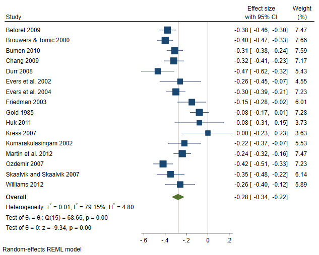
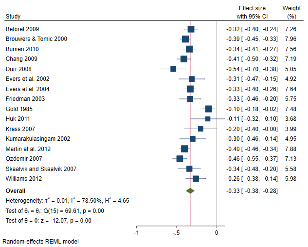
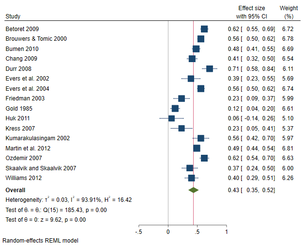
The overall (mean) correlations between CMSE and EE, DP, and LPA are –0.28, –0.33, and 0.43, respectively. The negative correlation between CMSE and both EE and DP suggests that a positive classroom experience leads to less EE and DP feelings. The scenario is reversed between CMSE and LPA (they are positively correlated), suggesting that a positive classroom experience will also lead to feeling more accomplished. From the plots, it seems there is considerable heterogeneity among studies, especially in the correlation between CMSE and the third dimension of burnout, LPA, where 10 out of the 16 studies had CIs that did not cross the overall effect vertical line.
You could also conduct univariate meta-regression of, say, y2 (correlation between CMSE and DP) on moderators such as percentage of female teachers (female_p) and publication type (pub_type) by typing
. frame fr_2: meta regress female_p i.pub_type
(output omitted)
Or perhaps construct a funnel plot to assess the small-study effect for variable y3:
. frame fr_3: meta funnelplot
(output omitted)
Performing a multivariate meta-analysis
The three separate meta-analyses do not account for the dependence between y1, y2, and y3. We will use the meta mvregress command to conduct a multivariate meta-analysis to pool the three-dimensional effect of burnout across studies while accounting for the dependence among the three outcomes. There are two components that contribute to the correlation among the effect sizes: the within-study correlation, which is accounted for by the six variables v11, v12, v13, v22, v23, and v33; and the between-study correlation, which is accounted for by the random-effects model (more specifically, by the covariance matrix of the random effects) that is assumed by default.
. meta mvregress y1 y2 y3, wcovvariables(v11 v12 v13 v22 v23 v33)

Performing EM optimization ...

Performing gradient-based optimization:
Iteration 0:   log restricted-likelihood =  37.738248
Iteration 1:   log restricted-likelihood =  40.417156
Iteration 2:   log restricted-likelihood =   40.56626
Iteration 3:   log restricted-likelihood =  40.567178
Iteration 4:   log restricted-likelihood =  40.567179

Multivariate random-effects meta-analysis       Number of obs     =         48
Method: REML                                    Number of studies =         16
                                                Obs per study:
                                                              min =          3
                                                              avg =        3.0
                                                              max =          3
                                                Wald chi2(0)      =          .
Log restricted-likelihood = 40.567179           Prob > chi2       =          .
| Coefficient Std. err. z P>|z| [95% conf. interval] | ||
| y1 | ||
| _cons | -.2773755 .0302203 -9.18 0.000 -.3366062 -.2181447 | |
| y2 | ||
| _cons | -.3285461 .0284353 -11.55 0.000 -.3842783 -.272814 | |
| y3 | ||
| _cons | .4331267 .0449928 9.63 0.000 .3449425 .521311 | |
| Random-effects parameters | Estimate | |
| Unstructured: | ||
| sd(y1) | .1066603 | |
| sd(y2) | .0992441 | |
| sd(y3) | .1708421 | |
| corr(y1,y2) | .8779874 | |
| corr(y1,y3) | -.9685017 | |
| corr(y2,y3) | -.876861 | |
More conveniently, you may express the above specification by using the stub shortcut notation:
. meta mvregress y*, wcovvariables(v*)
(output omitted)
The first table displays the overall trivariate correlation from the multivariate model. The estimates are very similar to the univariate ones reported on the forest plots. This is often the case, especially when no missing data are reported by the studies (which is our case). Whenever studies report missing values on some outcome of interest, multivariate meta-analysis can, by observing related outcomes, borrow strength from these outcomes to produce more efficient overall estimates for all outcomes. The three overall correlations are significant, suggesting that EE, DP, and LPA all relate to CMSE.
The multivariate homogeneity test, which tests whether the trivariate correlation is constant across studies, is rejected (p < 0.00001). The second table shows the standard deviations and correlations of the random effects.
The default model assumed by meta mvregress is a random-effects model with an unstructured covariance matrix for the random effects and is fit via restricted maximum-likelihood estimation (REML). You may use the random() option to request other settings. For example, below we specify a random-effects model with an exchangeable covariance structure for the random effects estimated via maximum likelihood estimation (MLE).
. meta mvregress y*, wcovvariables(v*) random(mle, covariance(exchangeable))

Performing EM optimization ...

Performing gradient-based optimization:
Iteration 0:   log likelihood =  35.789919
Iteration 1:   log likelihood =  36.294019
Iteration 2:   log likelihood =  36.298873
Iteration 3:   log likelihood =  36.298874

Multivariate random-effects meta-analysis       Number of obs     =         48
Method: ML                                      Number of studies =         16
                                                Obs per study:
                                                              min =          3
                                                              avg =        3.0
                                                              max =          3
                                                Wald chi2(0)      =          .
Log likelihood = 36.298874                      Prob > chi2       =          .
| Coefficient Std. err. z P>|z| [95% conf. interval] | ||
| y1 | ||
| _cons | -.2812558 .0312227 -9.01 0.000 -.3424512 -.2200604 | |
| y2 | ||
| _cons | -.2812558 .0312227 -9.01 0.000 -.3424512 -.2200604 | |
| y3 | ||
| _cons | .4406485 .0308653 14.28 0.000 .3801536 .5011434 | |
| Random-effects parameters | Estimate | |
| Exchangeable: | ||
| sd(y1 y2 y3) | .1103228 | |
| corr(y1 y2 y3) | -.4598057 | |
The first table shows similar values to the overall trivariate correlation from the previous REML model. The second table displays the assumed common value of the random-effects standard deviation (0.1103) and the assumed common correlation among the random effects (–0.4598).
You could also specify random(jwriley) to request the Jackson—White—Riley noniterative method for estimating the between-study random-effects covariance matrix. The method can be seen as a multivariate extension of the popular univariate method of DerSimonian and Laird.
If you wish to assume a fixed-effects multivariate MA model, you may specify option fixed:
. meta mvregress y*, wcovvariables(v*) fixed
(output omitted)
Assessing multivariate heterogeneity
Upon successfully fitting your multivariate model, you may explore the heterogeneity among the correlated effect sizes across the studies via the estat heterogeneity postestimation command:
. quietly meta mvregress y*, wcovvariables(v*)

. estat heterogeneity

Method: Cochran
Joint:
  I2 (%) = 82.47
      H2 =  5.71

Method: Jackson–White–Riley
y1:
  I2 (%) = 82.37
       R =  2.38

y2:
  I2 (%) = 83.92
       R =  2.49

y3:
  I2 (%) = 94.52
       R =  4.27

Joint:
  I2 (%) = 77.06
       R =  2.09
The Cochran heterogeneity statistics quantify the amount of heterogeneity jointly for all outcomes. \( I^2\) = 82.47% means that roughly 82% of the variability among the effect sizes across the studies is due to true heterogeneity between the studies as opposed to the sampling variability. The Jackson—White—Riley statistics quantify the amount of heterogeneity separately for each outcome variable and jointly for all outcomes. For instance, we saw from the forest plot of variable y3 (the correlation between CMSE and LPA) that there was considerable heterogeneity because of the many nonoverlapping study CIs. This is confirmed by the highest \( I^2\) value (roughly 95%) corresponding to outcome y3.
You can also use the Jackson—White—Riley statistics to assess heterogeneity jointly for a subset of dependent variables.. estat heterogeneity, jwriley(y1 y2)
Method: Jackson–White–Riley
y1 y2:
I2 (%) = 76.23
R = 2.05
The value of \( I^2\) is roughly 76%, which suggests that, when considered as a pair, the effect sizes in variables y1 and y2 are less variable than the individual effect sizes, albeit with considerable heterogeneity still present.
Predicting random effects and more
Various standard postestimation tools—such as predict, margins, and test—are also available after you fit a multivariate meta-analysis model. Below, we predict random effects by using predict, reffects, and we obtain their standard errors by specifying the reses() option.
. predict double re*, reffects reses(re_se*)

. set linesize 90

. list re*
| re1 re2 re3 re_se1 re_se2 re_se3 | |
| 1. | -.10283588 -.03131996 .17620617 .09978001 .0901633 .16225359 |
| 2. | -.09379568 -.05495025 .12575747 .09988817 .09205702 .16277886 |
| 3. | -.02938791 -.01429996 .0458616 .09973658 .09082035 .16198752 |
| 4. | -.00674903 -.04699805 -.02200034 .098104 .08902432 .16011173 |
| 5. | -.15505505 -.14830599 .25088819 .09530048 .08396402 .15573488 |
| 6. | .02059561 .01613239 -.03490522 .09268252 .08009149 .15180802 |
| 7. | -.05697903 -.02027662 .12091516 .09937867 .09083816 .16232895 |
| 8. | .09958159 .04976988 -.16574508 .09476274 .08488424 .15428564 |
| 9. | .18321031 .19925303 -.29725953 .09895307 .09032536 .16101285 |
| 10. | .1637504 .14524732 -.27103958 .08737944 .07581568 .14315724 |
| 11. | .1196294 .08084109 -.18393054 .0898793 .07911838 .14714454 |
| 12. | -.03289968 -.0253095 .07421782 .09507486 .08363428 .15483541 |
| 13. | -.00577343 -.07779175 .04872011 .09989025 .09205789 .16304962 |
| 14. | -.12152979 -.11379705 .18690794 .09933887 .08977333 .1614794 |
| 15. | -.00072944 .00359832 -.02299691 .09546701 .08470254 .15506071 |
| 16. | .01896759 .0382071 -.03159726 .09648813 .08623672 .15749337 |
Each row of predicted random effects represents the study-specific deviations from the mean trivariate correlation. Instead of the reses() option, you could have specified the revce() option to compute the full variance—covariance matrix of the predicted random effects in lieu of standard errors only.
Fitting a multivariate meta-regression (moderator analysis)
We can try to explain some of the heterogeneity highlighted in the univariate forest plots but also in the multivariate homogeneity test by performing a multivariate meta-regression using the variable pub_year (centered around year 2000). Perhaps newer studies report different magnitudes of the three outcomes compared with older studies, which might explain the discrepancies between the trivariate correlations across the studies. We simply incorporate our moderator by specifying it on the right-hand side of the equals sign, as follows:
. set linesize 80

. meta mvregress y* = pub_year, wcovvariables(v*) variance

Performing EM optimization ...

Performing gradient-based optimization:
Iteration 0:   log restricted-likelihood =  26.721723
Iteration 1:   log restricted-likelihood =   28.24878
Iteration 2:   log restricted-likelihood =   28.36236
Iteration 3:   log restricted-likelihood =  28.362971
Iteration 4:   log restricted-likelihood =  28.362971

Multivariate random-effects meta-regression     Number of obs     =         48
Method: REML                                    Number of studies =         16
                                                Obs per study:
                                                              min =          3
                                                              avg =        3.0
                                                              max =          3
                                                Wald chi2(3)      =       7.36
Log restricted-likelihood = 28.362971           Prob > chi2       =     0.0613
| Coefficient Std. err. z P>|z| [95% conf. interval] | ||
| y1 | ||
| pub_year | -.0050658 .0044898 -1.13 0.259 -.0138657 .003734 | |
| _cons | -.2495888 .0382269 -6.53 0.000 -.3245121 -.1746654 | |
| y2 | ||
| pub_year | -.0079188 .0034126 -2.32 0.020 -.0146074 -.0012302 | |
| _cons | -.2903522 .0292901 -9.91 0.000 -.3477597 -.2329446 | |
| y3 | ||
| pub_year | .0085855 .0066232 1.30 0.195 -.0043957 .0215666 | |
| _cons | .3873665 .056148 6.90 0.000 .2773184 .4974147 | |
| Random-effects parameters | Estimate | |
| Unstructured: | ||
| var(y1) | .010966 | |
| var(y2) | .0058382 | |
| var(y3) | .0267623 | |
| cov(y1,y2) | .007134 | |
| cov(y1,y3) | -.0164038 | |
| cov(y2,y3) | -.0107893 | |
We used option variance to report variances and covariances of random effects instead of standard deviations and correlations. The slope of pub_year for outcome y2 (–0.008) is significant and suggests that newer studies report smaller correlations between CMSE and DP. If we compare the random-effects table with the one from the constant-only model above, it seems that the moderator explained some of the between-studies variability for outcome y2: var(y2) went from 0.0098 (in the constant-only model) to 0.0058. However, the residual homogeneity test (p < 0.0001) suggests there is still a considerable amount of residual heterogeneity (remaining heterogeneity not explained by moderators). This is also confirmed if we type
. estat heterogeneity

Method: Cochran
Joint:
  I2 (%) = 79.39
      H2 =  4.85

Method: Jackson–White–Riley
y1:
  I2 (%) = 83.35
       R =  2.45

y2:
  I2 (%) = 77.81
       R =  2.12

y3:
  I2 (%) = 94.42
       R =  4.23

Joint:
  I2 (%) = 75.67
       R =  2.03
Notice that there was a reduction (from 83.92% for the constant-only model to 77.81%) in the Jackson—White—Riley \( I^2\) statistic corresponding to outcome y2 but the other values of the \( I^2\) statistic corresponding to y1 and y3 remained nearly the same.
References
Aloe, A. M., L. C. Amo, and M. E. Shanahan. 2014. Classroom management self-efficacy and burnout: A multivariate meta-analysis. Educational Psychology Review 26: 101–126.
Emmer, E. T. 1990. A scale for measuring teacher efficacy in classroom management and discipline. Paper presented at the annual meeting of the American Educational Research Association, Boston, MA.
Emmer, E. T., and J. Hickman. 1991. Teacher efficacy in classroom management and discipline. Educational and Psychological Measurement 51: 755–765. doi:10.1177/0013164491513027.
— by Houssein Assaad
Principal Statistician and Software Developer


