

In the spotlight: Using Python within Stata
Did you know that you can use Python within Stata? Well, you can—you can use Python from within Stata to access data with Internet API calls, process JSON data, create three-dimensional graphics, use machine learning and artificial intelligence algorithms to find patterns in your data, and much more. And the best part is that you can seamlessly move between Stata and Python to perform tasks such as these right alongside the analyses that you already perform using Stata.
I recently started writing a series of blog posts to help you get started using Python from within Stata. The first post shows you how to set up Stata to use Python, and the other posts help you get started with Python and then demonstrate interesting ways you can use it. Before you read the blog posts, I want to show you one way that you can take advantage of the Python integration in Stata. Here I use Stata to estimate marginal predictions from a logistic regression model and then Python to create a three-dimensional surface plot of those predictions.
I first fit a logistic regression model using data from the National Health and Nutrition Examination Survey (NHANES). The dependent variable, highbp, is an indicator for high blood pressure, and I included the main effects and interaction of the continuous variables age and weight.
. webuse nhanes2, clear

. svy: logistic highbp c.age##c.weight
(running logistic on estimation sample

Survey: Logistic regression

Number of strata   =        31                Number of obs     =       10,351
Number of PSUs     =        62                Population size   =  117,157,513
                                              Design df         =           31
                                              F(   3,     29)   =       418.97
                                              Prob > F          =       0.0000
| Linearized | ||
| highbp | Odds Ratio Std. Err. t P>|t| [95% Conf. Interval] | |
| age | 1.100678 .0088786 11.89 0.000 1.082718 1.118935 | |
| weight | 1.07534 .0063892 12.23 0.000 1.062388 1.08845 | |
| c.age#c.weight | .9993975 .0001138 -5.29 0.000 .9991655 .9996296 | |
| _cons | .0002925 .0001194 -19.94 0.000 .0001273 .0006724 | |
The estimated odds ratio for the interaction of age and weight is 0.9994, and the p-value for the estimate is 0.000. Interpreting this result is challenging because the odds ratio is essentially equal to the null value of 1, but the p-value is essentially 0. Is the interaction effect meaningful? It is often easier to determine this by looking at the predicted probability of the outcome at different levels of the covariates rather than looking only at this odds ratio.
The code block below uses margins to estimate the predicted probability of hypertension for all combinations of age and weight for values of age ranging from 20 to 80 years in increments of 5 and for values of weight ranging from 40 to 180 kilograms in increments of 5. The option saving(predictions, replace) saves the predictions to a dataset named predictions. I then use the dataset predictions, rename three variables in the dataset, and save it again.
webuse nhanes2, clear
svy: logistic highbp age weight c.age#c.weight
quietly margins, at(age=(20(5)80) weight=(40(5)180))
                 vce(unconditional) saving(predictions, replace)
use predictions, clear
rename _at1 age
rename _at2 weight
rename _margin pr_highbp
save predictions, replace
In a previous Stata News article, I used graph twoway contour to create a contour plot of the predicted probability of hypertension saved in predictions. Today, I'm going to use Python to create a three-dimensional surface plot of the predicted probability.
You can run the Python code below in a Stata do-file after you have set up Stata to use Python. The Python code block begins with python: and ends with end. I have included comments in the Python code to give you clues about the purpose of each collection of Python statements. You can read a detailed explanation of the Python code at the Stata Blog.
python:
# Import the necessary Python packages
import numpy as np
import pandas as pd
import matplotlib
import matplotlib.pyplot as plt
matplotlib.use('TkAgg')
# Read (import) the Stata dataset "predictions.dta"
# into a pandas data frame named "data"
data = pd.read_stata("predictions.dta")
# Define a 3-D graph named "ax"
ax = plt.axes(projection='3d')
# Specify the axis ticks
ax.set_xticks(np.arange(20, 100, step=10))
ax.set_yticks(np.arange(40, 220, step=40))
ax.set_zticks(np.arange( 0, 1, step=0.2))
# Specify the title and axis titles
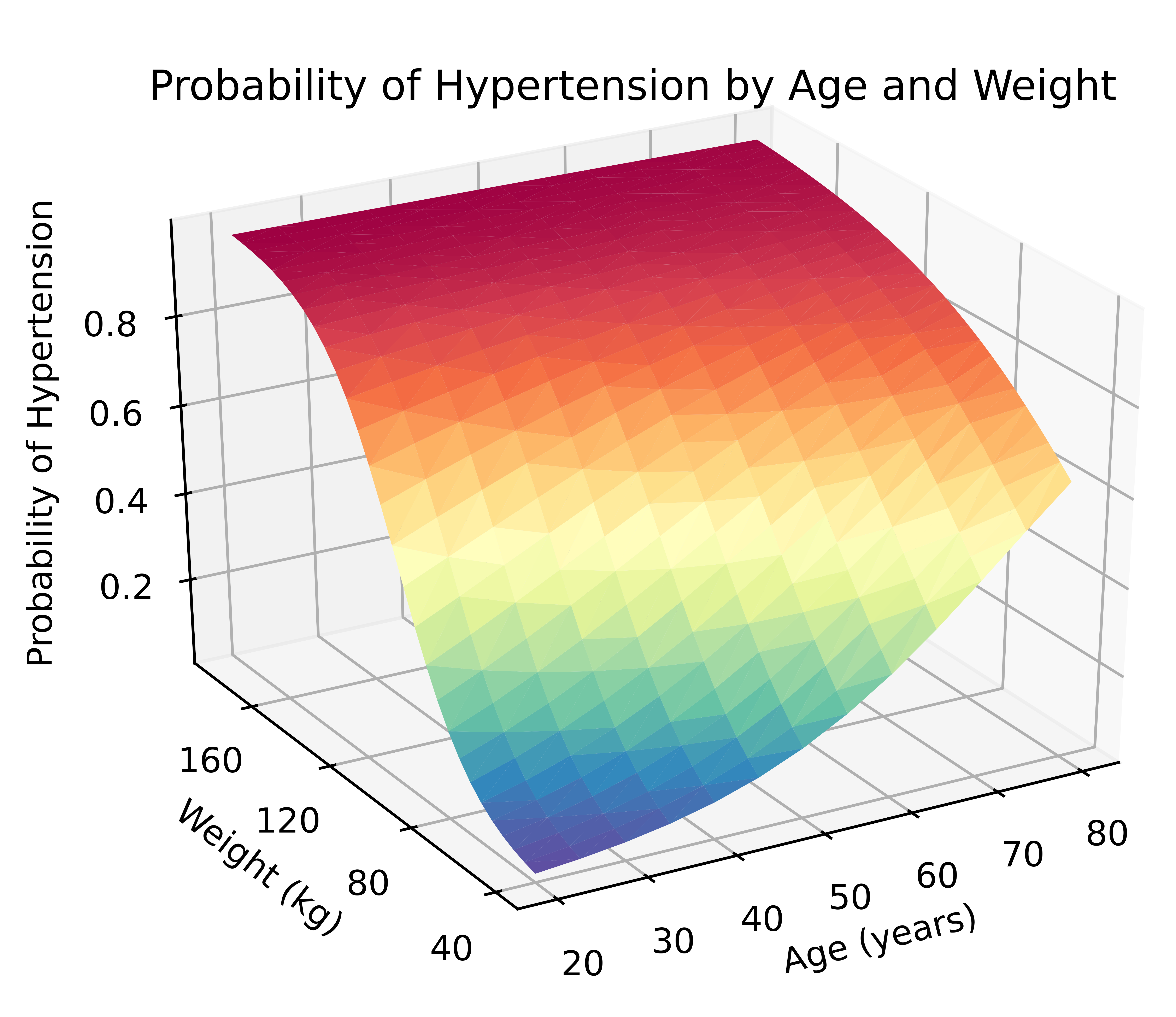
ax.set_title("Probability of Hypertension by Age and Weight")
ax.set_xlabel("Age (years)")
ax.set_ylabel("Weight (kg)")
ax.zaxis.set_rotate_label(False)
ax.set_zlabel("Probability of Hypertension", rotation=90)
# Specify the view angle of the graph
ax.view_init(elev=30, azim=240)
# Render the graph
ax.plot_trisurf(data['age'], data['weight'], data['pr_highbp'],
cmap=plt.cm.Spectral_r,
edgecolor='none')
# Save the graph
plt.savefig("Margins3d_3.png", dpi=1200)
end
The resulting three-dimensional surface plot shows the predicted probability of hypertension for values of age and weight and allows us to visualize their interaction. The probabilities are indicated by the height of the surface on the z axis and by the color of the surface. Blue indicates lower probabilities of hypertension, and red indicates higher probabilities of hypertension.
All the Stata commands and Python code in this example can be run in the same do-file. And three-dimensional surface plots are just one of the many fun things you can do with Stata and Python.
Ready to try it for yourself? My blog posts will show you how to get started:
- Setting up Stata to use Python
- Three ways to use Python in Stata
- How to install Python packages
- How to use Python packages
- Three-dimensional surface plots of marginal predictions
- Using APIs and JSON data with Python
- Machine learning and artificial intelligence with Python
Stay tuned into the Stata Blog for more posts on exciting ways to use Python within Stata. And even better, explore ways to take advantage of Stata/Python integration in your own research.
— Chuck Huber
Director of Statistical Outreach


