

In the spotlight: Fun with frames
Stata 16 lets you use multiple datasets simultaneously with frames. I have written a blog post to show you some of the fun things you can do with frames, and there is a detailed introduction to frames in the Stata 16 manual that will make you an expert. This article will show you a quick example that I hope will inspire you to learn more about this powerful new feature.
Let's begin by using frame create to create a new data frame named patients. Next, we can use frame change to change to the patient frame. Then, we can type webuse nhanes2 to use the NHANES II dataset in the data frame patients.
. frame create patients
. frame change patients
. webuse nhanes2
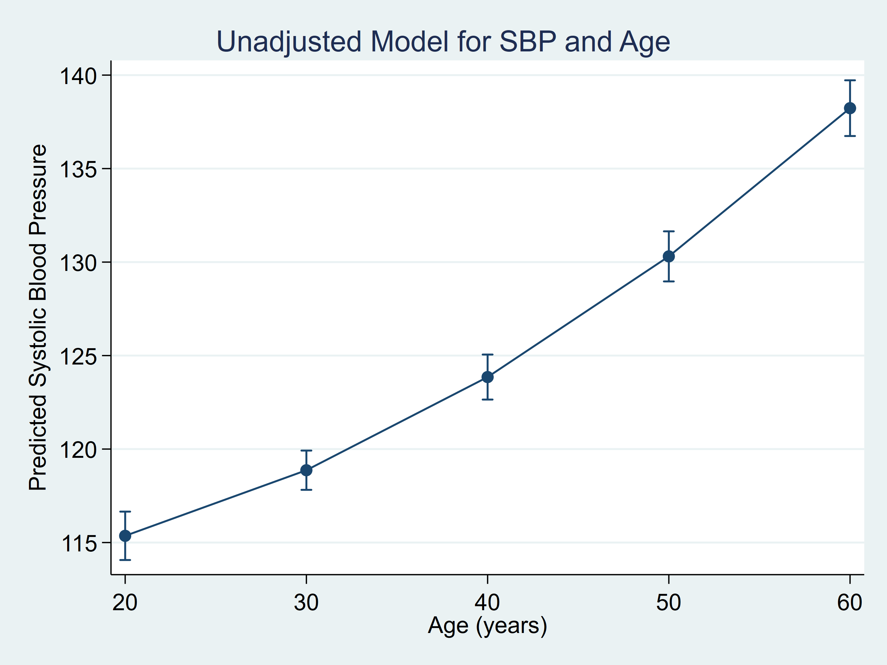
Let's fit a linear regression model for the dependent variable systolic blood pressure (bpsystol) and include age and age-squared (c.age##c.age) as independent variables. I have included the svy linearized: prefix to account for the survey weights in the dataset. Then, I use margins to estimate predicted systolic blood pressure (SBP) at age 20–60 in increments of 10. Note that I included the option saving(pr_unadj, replace) to save the marginal predictions to a dataset named pr_unadj. Then, I use marginsplot to graph the marginal predictions. I have omitted the graph options from marginsplot to keep the syntax simple. And I refer to this model as the "unadjusted" model because the model does not include other covariates.
. svy linearized: regress bpsystol c.age##c.age
. margins, at(age=(20(10)60)) saving(pr_unadj, replace)
. marginsplot, ...
Figure 1: marginsplot for predicted SBP by age
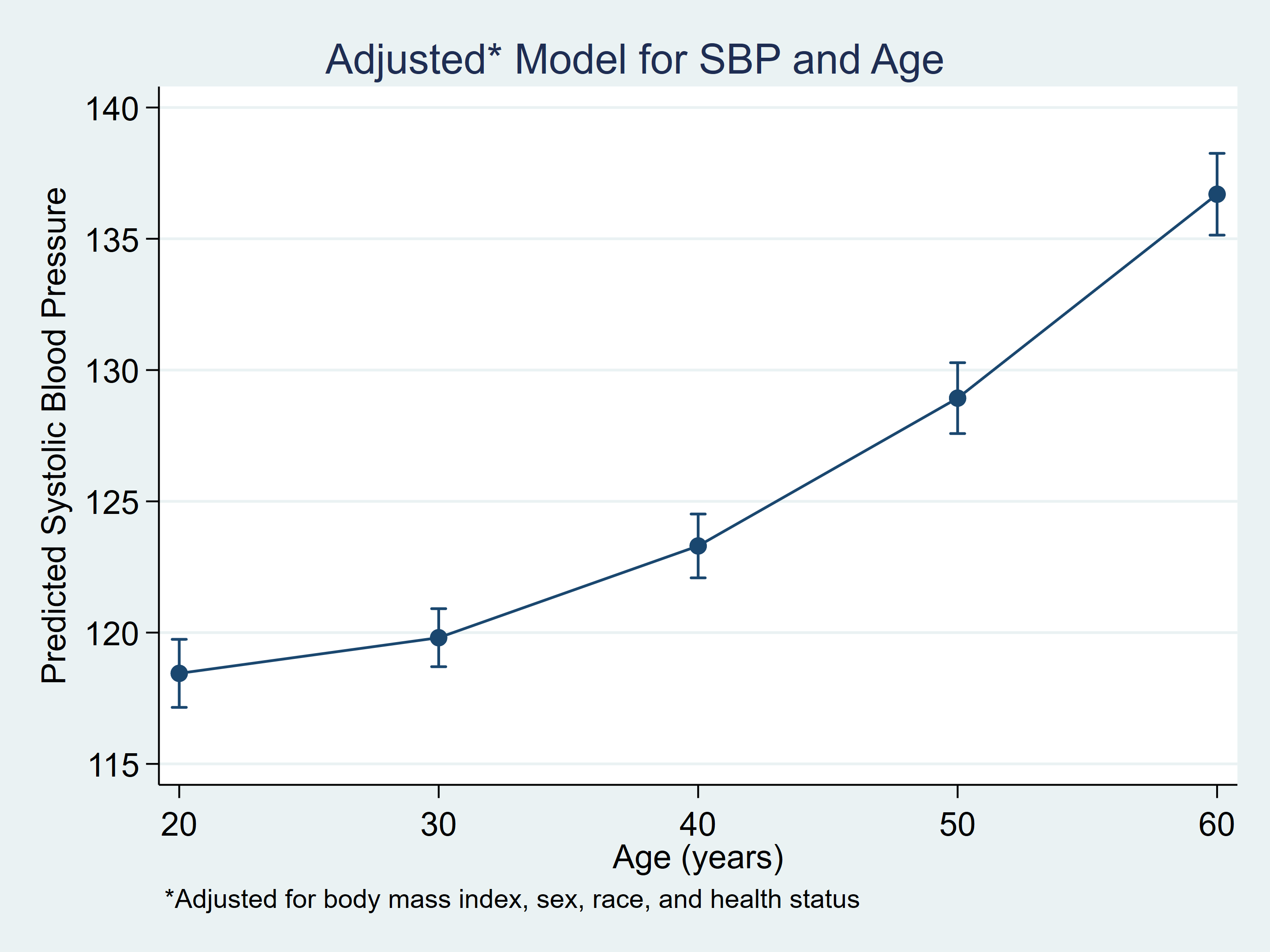
Let's fit a second model that adjusts our model for the effects of body mass index (BMI), sex, race, and health status. And I refer to this model as the "adjusted" model because the model includes other covariates.
. svy linearized: regress bpsystol c.age##c.age bmi c.age##c.bmi i.sex i.race i.hlthstat
. margins, at(age=(20(10)60)) saving(pr_adj, replace)
. marginsplot, ...
Figure 2: marginsplot for predicted SBP by age adjusted for covariates
The marginsplots look similar but slightly different. It would be nice to see the predictions in the same graph. This is easy using frames. Let's begin by creating a new data frame named unadjusted, change to that frame, and open the dataset named pr_unadj, which contains the marginal predictions from our unadjusted model above.
. frame create unadjusted
. frame change unadjusted
. use pr_unadj
This dataset includes the variables
. describe _at1 _margin _ci_lb _ci_ub
| variable name storage type display format value label variable label |
| _at1 byte %9.0g age in years |
| _margin float %9.0g Linear prediction, predict() |
| _ci_lb float %9.0g 95% Confidence interval, LB |
| _ci_ub float %9.0g 95% Confidence interval, UB |
Let's change the variable names to make them easier to recognize and save the data. We use the variable labels as a guide.
. rename _at1 age
. rename _margin unadj_pr
. rename _ci_lb unadj_lb
. rename _ci_ub unadj_ub
. save pr_unadj, replace
. list age unadj_pr unadj_lb unadj_ub
| age unajd_pr unadj_lb unadj_ub | |
| 1. | 20 115.4 114.1 116.7 |
| 2. | 30 118.9 117.8 119.9 |
| 3. | 40 123.9 122.6 125.1 |
| 4. | 50 130.3 129.0 131.6 |
| 5. | 60 138.2 136.7 139.7 |
Let's create another data frame named adjusted and repeat the same process for the predictions from our adjusted model.
. frame create adjusted
. frame change adjusted
. use pr_adj
. rename _at1 age
. rename _margin adj_pr
. rename _ci_lb adj_lb
. rename _ci_ub adj_ub
. save pr_adj, replace
. list age adj_pr adj_lb adj_ub
| age ajd_pr adj_lb adj_ub | |
| 1. | 20 118.4 117.2 119.7 |
| 2. | 30 119.8 118.7 120.9 |
| 3. | 40 123.3 122.1 124.5 |
| 4. | 50 128.9 127.6 130.3 |
| 5. | 60 136.7 135.1 138.3 |
Now, we can use frlink to link the two data frames using age as the linking variable. And we can use frget to include the variables unadj_pr, unadj_lb, and unadj_ub from the data frame unadjusted.
. frlink 1:1 age, frame(unadjusted)
. frget unadj_pr unadj_lb unadj_ub, from(unadjusted)
All the marginal predictions along with their confidence bounds from both models are now in the data frame adjusted.
. list age unadj_pr unadj_lb unadj_ub adj_pr adj_lb adj_ub
| age unadj_pr unadj_lb unadj_ub adj_pr adj_lb adj_ub | |
| 1. | 20 115.4 114.1 116.7 118.4 117.2 119.7 |
| 2. | 30 118.9 117.8 119.9 119.8 118.7 120.9 |
| 3. | 40 123.9 122.6 125.1 123.3 122.1 124.5 |
| 4. | 50 130.3 129.0 131.6 128.9 127.6 130.3 |
| 5. | 60 138.2 136.7 139.7 136.7 135.1 138.3 |
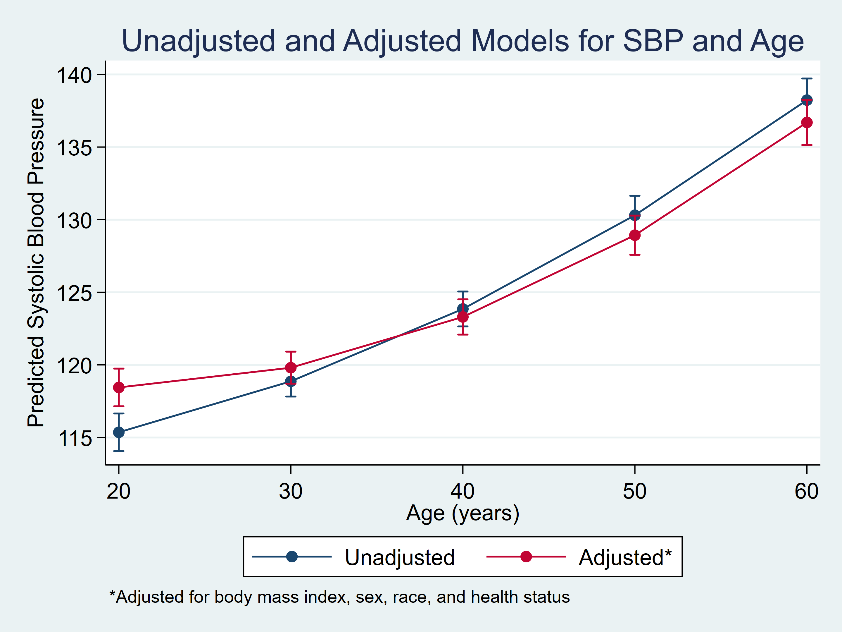
And we can use twoway to graph the marginal predictions from both our unadjusted and adjusted models.
. twoway (connected unadj_pr age , lcolor(navy))
(rcap unadj_ub unadj_lb age, lcolor(navy))
(connected adj_pr age , mcolor(cranberry) lcolor(cranberry))
(rcap adj_ub adj_lb age , lcolor(cranberry)), ...
Figure 3: marginsplot for the unadjusted and adjusted models
You can learn more about frames in the manual, and you can see more examples in my recent blog post, Fun with Frames.
— Chuck Huber
Associate Director of Statistical Outreach


