

In the spotlight: Uncovering unobserved groups in your data with fmm
Often, data come from distinct and observable groups such as males and females, single and married, or new and old manufacturing processes. If these groups behave differently, we observe heterogeneity in the data.
But in many cases we cannot observe groups directly. Examples include individuals with good and poor health, risk-averse and risk-seeking investors, and apples from different orchards.
Here I show one way of addressing unobserved heterogeneity with finite mixture models.
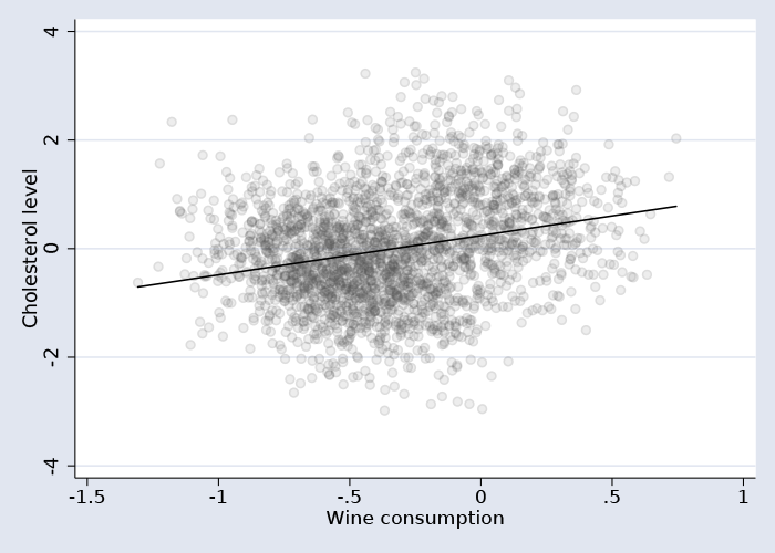
We have data on individuals' standardized cholesterol levels (chol) and their mean-centered monthly red wine consumption (wine).
A linear fit line superimposed on the scatterplot of the data suggests there is a positive relationship between the two.
And a simple regression model confirms the positive relationship.
. regress chol wine
| chol | Coef. Std. Err. t P>|t| [95% Conf. Interval] | |
| wine | .7243775 .0553511 13.09 0.000 .6158387 .8329162 | |
| _cons | .2408989 .0267081 9.02 0.000 .1885266 .2932712 | |
Let's see what happens when we add to our model a variable recording whether either parent had high cholesterol (pchol).
. regress chol wine pchol
| chol | Coef. Std. Err. t P>|t| [95% Conf. Interval] | |
| wine | -.1469443 .0632583 -2.32 0.020 -.2709885 -.0229001 | |
| pchol | .5037735 .0221205 22.77 0.000 .4603971 .54715 | |
| _cons | -.0488678 .0274366 -1.78 0.075 -.1026686 .004933 | |
Now we find that wine consumption has a slight negative effect on cholesterol and that parents' cholesterol has a positive effect.
We hypothesize that an individual may inherit a "high cholesterol" gene and that we have two types of individuals in the population—those with the cholesterol gene and those without. However, we do not know who belongs to each group.
We use fmm to probabilistically classify the sample into groups. By adding the fmm prefix followed by 2, we indicate that we want to fit a model for two underlying subpopulations. We use the lcprob(pchol) option to include parents' cholesterol history as the predictor of the unobserved group, also called the latent class.
. fmm 2, lcprob(pchol): regress chol wine
The output below shows a regression model for each class. Wine consumption has a negative effect on cholesterol level in each class.
Class          : 1
Response       : chol
Model          : regress
| Coef. Std. Err. z P>|z| [95% Conf. Interval] | ||
| chol | ||
| wine | -.6850974 .0783981 -8.74 0.000 -.8387549 -.5314399 | |
| _cons | -.7401758 .0443478 -16.69 0.000 -.8270959 -.6532557 | |
| var(e.chol) | .6152073 .0219867 .5735887 .6598457 | |
| Coef. Std. Err. z P>|z| [95% Conf. Interval] | ||
| chol | ||
| wine | -.4798618 .1319125 -3.64 0.000 -.7384056 -.221318 | |
| _cons | .8343004 .0323813 25.76 0.000 .7708342 .8977667 | |
| var(e.chol) | .6720669 .0383181 .601009 .7515261 | |
The table below gives the coefficients for the latent class membership on the logit scale.
| Coef. Std. Err. z P>|z| [95% Conf. Interval] | ||
| 1.Class | (base outcome) | |
| 2.Class | ||
| pchol | 7.473592 .8977705 8.32 0.000 5.713994 9.23319 | |
| _cons | -3.228661 .3939579 -8.20 0.000 -4.000804 -2.456518 | |
We use estat lcprob to display marginal class probabilities on the probability scale.
. estat lcprob
| Delta-method | ||
| Margin Std. Err. [95% Conf. Interval] | ||
| Class | ||
| 1 | .6743291 .0055936 .6632719 .6851956 | |
| 2 | .3256709 .0055936 .3148044 .3367281 | |
About 67% of individuals are expected to be in group 1 and 33% in group 2. But which group is which? To find out, we use estat lcmean to calculate the marginal means for each class. The reported mean for class 1 is lower than the reported mean for class 2. Therefore, class 1 corresponds to individuals with no cholesterol gene, and class 2 to those with the gene.
. estat lcmean
| Delta-method | ||
| Margin Std. Err. z P>|z| [95% Conf. Interval] | ||
| 1 | ||
| chol | -.5123399 .024033 -21.32 0.000 -.5594438 -.465236 | |
| 2 | ||
| chol | .9938833 .0601744 16.52 0.000 .8759435 1.111823 | |
We can even classify the individuals in our dataset into the two groups by predicting posterior latent-class probabilities and using a cutpoint (we will use 0.5) to assign each observation to a group.
. predict c1, classposteriorpr

. summarize c1
| Variable | Obs Mean Std. Dev. Min Max | |
| c1 | 2,500 .6743291 .4538173 6.22e-09 1 | |
| lgroup | Freq. Percent Cum. | |
| 0 | 1,690 67.60 67.60 | |
| 1 | 810 32.40 100.00 | |
| Total | 2,500 100.00 | |
From the tabulation of predicted group membership, we see that our classification is close to the output produced by estat lcprob above.
Finally, we draw a scatterplot with the linear fit line for each group.
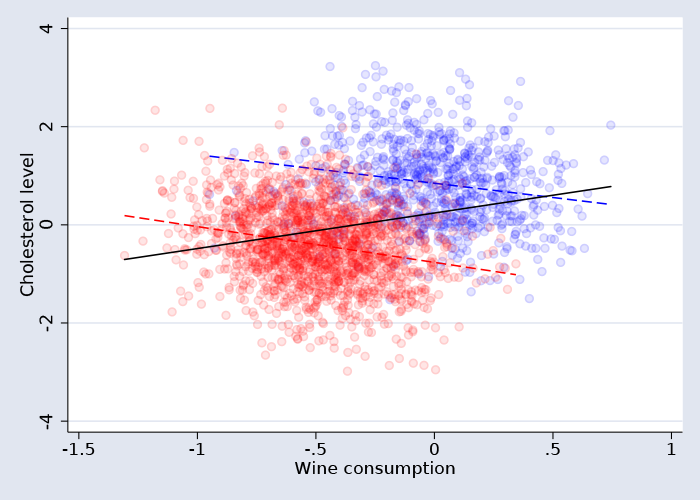
Some of you may recognize this graph as an illustration of Simpson's paradox, where a trend present in the data reverses when the data are divided into subgroups.
— Rafal Raciborski
Senior Statistical Developer


