Postestimation Selector

Let's see it work

Suppose we have just fit a linear regression of systolic blood pressure on age, weight, and an indicator for females.

. webuse nhanes2, clear

. regress bpsystol age weight i.sex


      Source 
 
       SS           df       MS  
   Number of obs   =    10,351
   F(3, 10347)     =   1501.75
       Model 
   1709209.9         3  569736.633
   Prob > F        =    0.0000
    Residual 
  3925460.13    10,347  379.381476
   R-squared       =    0.3033
   Adj R-squared   =    0.3031
       Total 
  5634670.03    10,350  544.412563
   Root MSE        =    19.478



    bpsystol 
 
 Coefficient  Std. err.      t    P>|t|     [95% conf. interval]

         age 
   .6374325   .0111334    57.25   0.000     .6156088    .6592562
      weight 
   .4170339    .013474    30.95   0.000     .3906221    .4434456
 
 
         sex 
                                                                
     Female  
   .8244702   .4140342     1.99   0.046     .0128832    1.636057
       _cons 
   70.13615   1.187299    59.07   0.000     67.80881    72.46348

What's next? How can we check to see whether any assumptions of the model have been violated? Can we compare the model we just fit to the more complex model we may have fit previously? Can we save our estimation results so that we can use them again later? How do we know which of Stata's hundreds, if not thousands, of postestimation features are available after the model we just fit?

The Postestimation Selector provides a list of all postestimation tools available after fitting our model and provides two-click access to the corresponding dialog boxes.

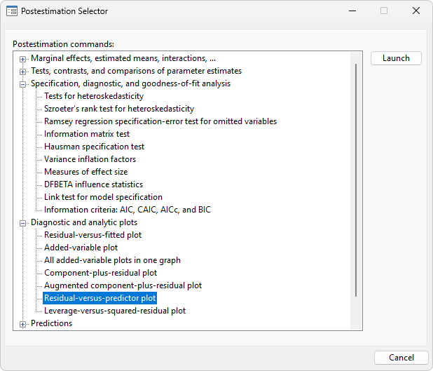
We have selected Residual-versus-predictor plot. We click on Launch, the dialog box opens, and we create our graph. The Postestimation Selector will remain open so that we can perform the rest of our analysis. For instance, we can select Tests for heteroskedasticity and open the dialog box to perform a Breusch–Pagan test.

We recommend that you leave the Postestimation Selector open at all times.

Next, we decide to fit a logistic regression model for highbp, a variable that is one when the subject's blood pressure is clinically high and is zero otherwise.

. logistic highbp age weight i.sex

Logistic regression                                    Number of obs =  10,351
                                                       LR chi2(3)    = 2326.44
                                                       Prob > chi2   =  0.0000
Log likelihood = -5887.5446                            Pseudo R2     =  0.1650


      highbp 
 
 Odds ratio   Std. err.      z    P>|z|     [95% conf. interval]

         age 
   1.052054   .0014852    35.95   0.000     1.049147    1.054969
      weight 
   1.044683    .001759    25.96   0.000     1.041242    1.048137
 
 
         sex 

     Female  
   1.036659   .0498306     0.75   0.454     .9434528    1.139074
       _cons 
    .002525   .0004077   -37.05   0.000     .0018401     .003465

Note: _cons estimates baseline odds.

As soon as our new model is estimated, the Postestimation Selector updates and shows us the postestimation tools that are now available.

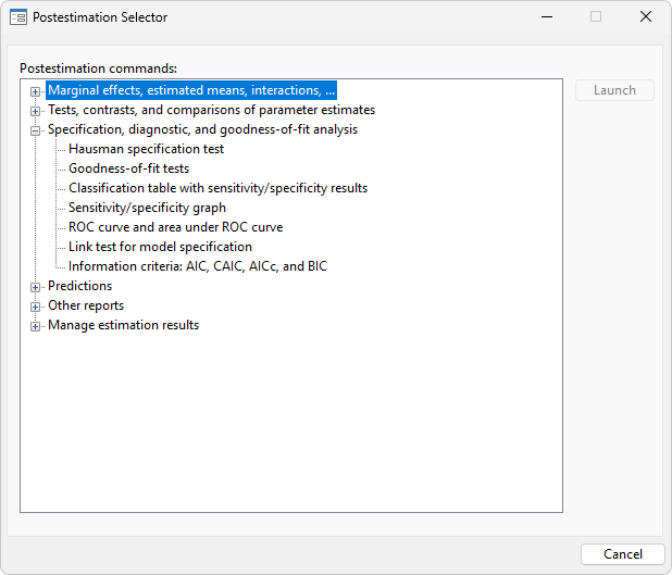
While we could have found a list of available postestimation commands from the help file for logistic postestimation, the Postestimation Selector is more specialized. It lists only postestimation features available for the exact model that was fit, adjusting for any options or prefixes that were specified. Notice what happens when we take into account the complex survey nature of this dataset by specifying the svy prefix with our command.

. svy: logistic highbp age weight i.sex
(running logistic on estimation sample)

Survey: Logistic regression

Number of strata = 31                            Number of obs   =      10,351
Number of PSUs   = 62                            Population size = 117,157,513
                                                 Design df       =          31
                                                 F(3, 29)        =      449.71
                                                 Prob > F        =      0.0000


             
 
             Linearized
      highbp 
 Odds ratio   std. err.      t    P>|t|     [95% conf. interval]

         age 
   1.054031   .0017933    30.93   0.000      1.05038    1.057695
      weight 
   1.046507   .0021333    22.30   0.000     1.042165    1.050867
 
 
         sex 

     Female  
   .9388421    .055388    -1.07   0.293      .832409    1.058884
       _cons 
   .0021719   .0004316   -30.86   0.000     .0014482    .0032572

Note: _cons estimates baseline odds.

We find that some of the diagnostics and goodness-of-fit statistics that were available previously are no longer listed and that there is a new list of postestimation features that are available only when fitting models to complex survey data.

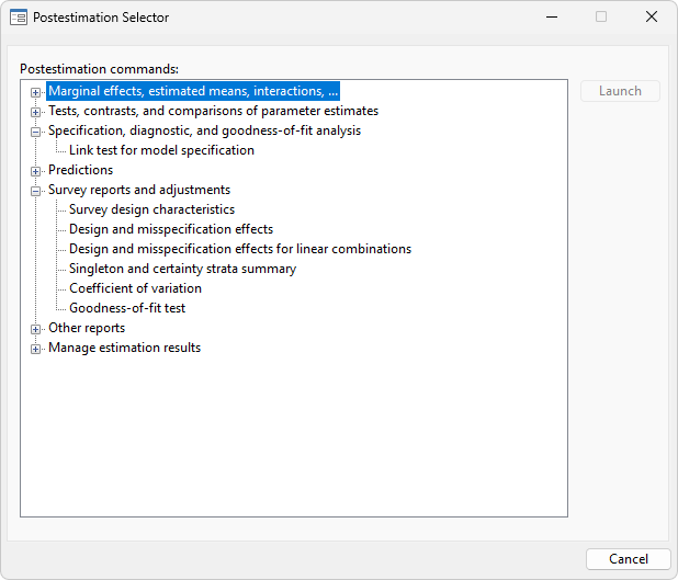
We can use the Postestimation Selector to guide us to the postestimation tools that are available after any model that we fit, and with any combinations of options or prefixes.