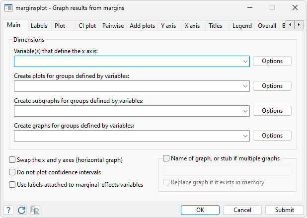
Stata makes it easy to graph statistics from fitted models using marginsplot. marginsplot graphs the results from margins, and margins itself can compute functions of fitted values after almost any estimation, linear or nonlinear.

Suppose we’ve just fit a two-way ANOVA of systolic blood pressure on age group, sex, and their interaction. We can estimate the response for each cell with margins:
. margins agegrp#sex

Adjusted predictions                                    Number of obs = 10,351
Model VCE: OLS

Expression: Linear prediction, predict()
| Delta-method | |||||||
| Margin std. err. t P>|t| [95% conf. interval] | |||||||
| agegrp#sex | |||||||
| 20-29#Male | 123.8862 .6052954 204.67 0.000 122.6997 125.0727 | ||||||
| 20-29 # | |||||||
| Female | 111.2849 .5827553 190.96 0.000 110.1426 112.4272 | ||||||
| 30-39#Male | 124.6818 .728709 171.10 0.000 123.2534 126.1102 | ||||||
| 30-39 # | |||||||
| Female | 116.2207 .692755 167.77 0.000 114.8627 117.5786 | ||||||
| 40-49#Male | 129.0033 .8187185 157.57 0.000 127.3984 130.6081 | ||||||
| 40-49 # | |||||||
| Female | 125.0468 .7859058 159.11 0.000 123.5063 126.5874 | ||||||
| 50-59#Male | 136.0864 .8241405 165.13 0.000 134.4709 137.7019 | ||||||
| 50-59 # | |||||||
| Female | 135.3164 .7703532 175.66 0.000 133.8064 136.8264 | ||||||
| 60-69#Male | 140.7451 .5465096 257.53 0.000 139.6738 141.8163 | ||||||
| 60-69 # | |||||||
| Female | 142.2368 .5236736 271.61 0.000 141.2103 143.2633 | ||||||
| 70+#Male | 146.3951 .9553456 153.24 0.000 144.5224 148.2678 | ||||||
| 70+#Female | 149.6599 .8717829 171.67 0.000 147.951 151.3687 | ||||||
To study the interaction it would be nice to see a graph. We use marginsplot:
. marginsplot

Variables that uniquely identify margins: agegrp sex
marginsplot automatically chooses the y-variable and x-variable and adds confidence intervals. We don’t have to stick with the defaults, though: marginsplot includes a rich set of options for changing axis definitions, labels, curves, confidence intervals, and more.
marginsplot also supports the features of the margins command, including the contrast operators. Let’s contrast women with men in each age group and plot the contrasts:
. margins r.sex@agegrp, contrast(nowald) Contrasts of adjusted predictions Number of obs = 10,351 Model VCE: OLS Expression: Linear prediction, predict(). marginsplot, yline(0) Variables that uniquely identify margins: agegrp
Delta-method Contrast std. err. [95% conf. interval] sex@agegrp (Female vs Male) 20-29 -12.60132 .8402299 -14.24833 -10.9543 (Female vs Male) 30-39 -8.461161 1.005448 -10.43203 -6.490288 (Female vs Male) 40-49 -3.956451 1.134878 -6.181031 -1.731871 (Female vs Male) 50-59 -.7699782 1.128119 -2.981309 1.441353 (Female vs Male) 60-69 1.491684 .756906 .0080022 2.975367 (Female vs Male) 70+ 3.264762 1.293325 .729594 5.79993
We see that systolic blood pressure is lower in younger women than in younger men. But among the old, the relationship is reversed, and women have higher blood pressure than men.
marginsplot works with nonlinear models, too. Suppose we've fit a logistic regression, modeling the probability of high blood pressure as a function of sex, age group, body mass index, and their interactions. marginsplot can contrast women with men on the probability scale:
. quietly margins r.sex, at(bmi=(10(1)65))

. marginsplot, xlabel(10(10)60) recast(line) recastci(rarea)

Variables that uniquely identify margins: bmi
We’ve only scratched the surface—anything that margins can compute, marginsplot can graph.