Stata fits fixed-effects (within), between-effects, random-effects (mixed), and correlated random-effects models on balanced and unbalanced data.
\(y[i,t] = X[i,t]b + u[i] + v[i,t]\)
That is, \(u[i]\) is the fixed or random effect and \(v[i,t]\) is the pure residual.
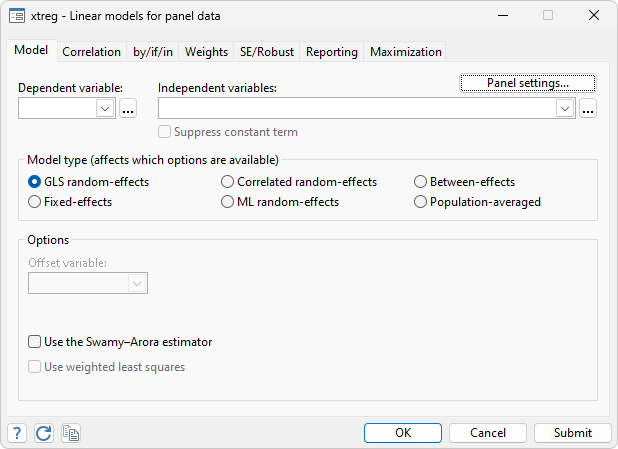
xtreg is Stata's feature for fitting linear models for panel data.
xtreg, fe estimates the parameters of fixed-effects models:
. webuse nlswork
(National Longitudinal Survey of Young Women, 14-24 years old in 1968)

. xtset

Panel variable: idcode (unbalanced)
 Time variable: year, 68 to 88, but with gaps
         Delta: 1 unit


. xtreg ln_w grade age c.age#c.age ttl_exp c.ttl_exp#c.ttl_exp tenure
     c.tenure#c.tenure 2.race not_smsa south, fe
note: grade omitted because of collinearity.
note: 2.race omitted because of collinearity.

Fixed-effects (within) regression                Number of obs     =     28,091
Group variable: idcode                           Number of groups  =      4,697

R-squared:                                       Obs per group:
     Within  = 0.1727                                          min =          1
     Between = 0.3505                                          avg =        6.0
     Overall = 0.2625                                          max =         15

                                                 F(8,23386)        =     610.12
corr(u_i, Xb) = 0.1936                           Prob > F          =     0.0000
| ln_wage | Coefficient Std. err. t P>|t| [95% conf. interval] | |
| grade | 0 (omitted) | |
| age | .0359987 .0033864 10.63 0.000 .0293611 .0426362 | |
| c.age#c.age | -.000723 .0000533 -13.58 0.000 -.0008274 -.0006186 | |
| ttl_exp | .0334668 .0029653 11.29 0.000 .0276545 .039279 | |
| c.ttl_exp# | ||
| c.ttl_exp | .0002163 .0001277 1.69 0.090 -.0000341 .0004666 | |
| tenure | .0357539 .0018487 19.34 0.000 .0321303 .0393775 | |
| c.tenure# | ||
| c.tenure | -.0019701 .000125 -15.76 0.000 -.0022151 -.0017251 | |
| race | ||
| Black | 0 (omitted) | |
| not_smsa | -.0890108 .0095316 -9.34 0.000 -.1076933 -.0703282 | |
| south | -.0606309 .0109319 -5.55 0.000 -.0820582 -.0392036 | |
| _cons | 1.03732 .0485546 21.36 0.000 .9421496 1.13249 | |
| sigma_u | .35562203 | |
| sigma_e | .29068923 | |
| rho | .59946283 (fraction of variance due to u_i) | |
We have used factor variables in the above example. The terms c.age#c.age, c.ttl_exp#c.ttl_exp, and c.tenure#c.tenure are just age-squared, total work experience-squared, and tenure-squared, respectively.
The syntax of all estimation commands is the same: the name of the dependent variable is followed by the names of the independent variables.
In this case, the dependent variable, ln_w (log of wage), was modeled as a function of a number of explanatory variables. Note that grade and black were omitted from the model because they do not vary within person.
Our dataset contains 28,091 “observations”, which are 4,697 people, each observed, on average, on 6.0 different years. An observation in our data is a person in a given year. The dataset contains variable idcode, which identifies the persons — the \(i\) index in \(X[i,t]\). Before fitting the model, we typed xtset to show that we had previously told Stata the panel variable. Told once, Stata remembers.
To fit the corresponding random-effects model, we use the same command but change the fe option to re.
. xtreg ln_w grade age c.age#c.age ttl_exp c.ttl_exp#c.ttl_exp tenure
     c.tenure#c.tenure 2.race not_smsa south, re

Random-effects GLS regression                   Number of obs     =     28,091
Group variable: idcode                          Number of groups  =      4,697

R-squared:                                      Obs per group:
     Within  = 0.1715                                         min =          1
     Between = 0.4784                                         avg =        6.0
     Overall = 0.3708                                         max =         15

                                                Wald chi2(10)     =    9244.74
corr(u_i, X) = 0 (assumed)                      Prob > chi2       =     0.0000
| ln_wage | Coefficient Std. err. z P>|z| [95% conf. interval] | |
| grade | .0646499 .0017812 36.30 0.000 .0611589 .0681409 | |
| age | .0368059 .0031195 11.80 0.000 .0306918 .0429201 | |
| c.age#c.age | -.0007133 .00005 -14.27 0.000 -.0008113 -.0006153 | |
| ttl_exp | .0290208 .002422 11.98 0.000 .0242739 .0337678 | |
| c.ttl_exp# | ||
| c.ttl_exp | .0003049 .0001162 2.62 0.009 .000077 .0005327 | |
| tenure | .0392519 .0017554 22.36 0.000 .0358113 .0426925 | |
| c.tenure# | ||
| c.tenure | -.0020035 .0001193 -16.80 0.000 -.0022373 -.0017697 | |
| race | ||
| Black | -.053053 .0099926 -5.31 0.000 -.0726381 -.0334679 | |
| not_smsa | -.1308252 .0071751 -18.23 0.000 -.1448881 -.1167622 | |
| south | -.0868922 .0073032 -11.90 0.000 -.1012062 -.0725781 | |
| _cons | .2387207 .049469 4.83 0.000 .1417633 .3356781 | |
| sigma_u | .25790526 | |
| sigma_e | .29068923 | |
| rho | .44045273 (fraction of variance due to u_i) | |
We can also perform the Hausman specification test, which compares the consistent fixed-effects model with the efficient random-effects model. To do that, we must first store the results from our random-effects model, refit the fixed-effects model to make those results current, and then perform the test.
. estimates store random_effects

. quietly xtreg ln_w grade age c.age#c.age ttl_exp c.ttl_exp#c.ttl_exp tenure
     c.tenure#c.tenure 2.race not_smsa south, fe

. hausman

. random_effects
| ||
| (b) (B) (b-B) sqrt(diag(V_b-V_B)) | ||
| . random_eff~s Difference Std. err. | ||
| age | .0359987 .0368059 -.0008073 .0013177 | |
| c.age#c.age | -.000723 -.0007133 -9.68e-06 .0000184 | |
| ttl_exp | .0334668 .0290208 .0044459 .001711 | |
| c.ttl_exp# | ||
| c.ttl_exp | .0002163 .0003049 -.0000886 .000053 | |
| tenure | .0357539 .0392519 -.003498 .0005797 | |
| c.tenure# | ||
| c.tenure | -.0019701 -.0020035 .0000334 .0000373 | |
| not_smsa | -.0890108 -.1308252 .0418144 .0062745 | |
| south | -.0606309 -.0868922 .0262613 .0081345 | |
We could alternatively perform a Mundlak specification test, which works after estimation with cluster–robust standard errors using estat mundlak.
In addition, Stata can perform the Breusch–Pagan Lagrange multiplier test for random effects and can calculate various predictions, including the random effect, based on the estimates.
Equally as important as its ability to fit statistical models with cross-sectional time-series data is Stata's ability to provide meaningful summary statistics.
xtsum reports means and standard deviations in a meaningful way:
. xtsum hours
| Variable | Mean Std. Dev. Min Max | Observations | ||
| hours overall | 36.55956 9.869623 1 168 | N = 28467 | ||
| between | 7.846585 1 83.5 | n = 4710 | ||
| within | 7.520712 -2.154726 130.0596 | T-bar = 6.04395 |
The negative minimum for hours within is not a mistake; the within shows the variation of hours within person around the global mean 36.55956.
xttab does the same for one-way tabulations:
. xttab msp

                  Overall             Between            Within
| msp | Freq. Percent Freq. Percent Percent | |
| 0 | 11324 39.71 3113 66.08 62.69 | |
| 1 | 17194 60.29 3643 77.33 75.75 | |
| Total | 28518 100.00 6756 143.41 69.73 | |
msp is a variable that takes on the value 1 if the surveyed woman is married and the spouse is present in the household. Overall, some 60% of our person-year observations are msp. Taking women individually, 66% of the women are at some point msp, and 77% are not; thus some women are msp one year and not others. Taking women one at a time, if a woman is ever msp, 55% of her observations are msp observations. If a woman is ever not msp, 72% of her observations are not msp. (If marital status never varied in our data, the within percentages would all be 100.)
xttrans reports the transition matrix:
. xttrans msp
| 1 if | married, | 1 if married, spouse | spouse | present | present | 0 1 | Total |
| 0 | 80.49 19.51 | 100.00 | 1 | 7.96 92.04 | 100.00 |
| Total | 37.11 62.89 | 100.00 |
Explore more longitudinal data/panel data features in Stata.


