Binary response models
One-parameter logistic (1PL)
Two-parameter logistic (2PL)
Three-parameter logistic (3PL)
Ordinal response models
Graded response
Partial credit
Rating scale
Categorical response models
Nominal response
Hybrid models with differing response types
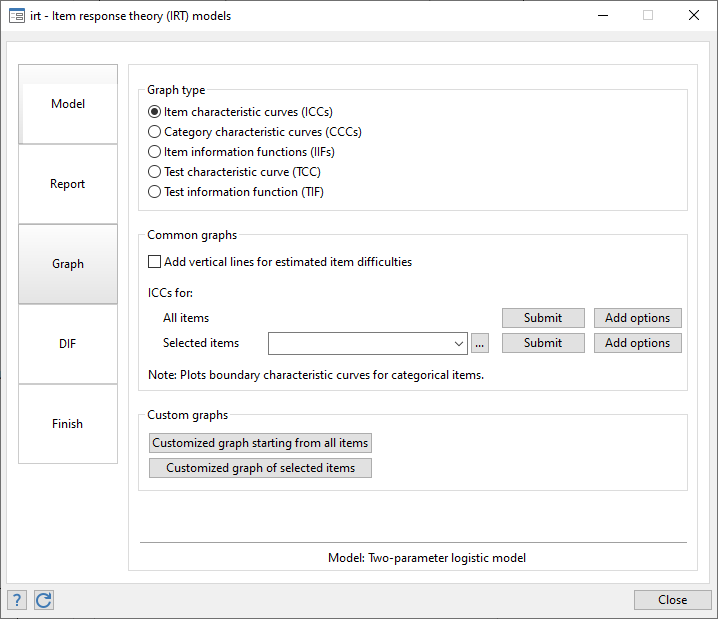
Graphs
Item characteristic curve
Test characteristic curve
Item information function
Test information function
Differential item functioning (DIF)
;)
Many researchers study cognitive abilities, personality traits, attitudes, quality of life, patient satisfaction, and other attributes that cannot be measured directly. To quantify these types of latent traits, a researcher often develops an instrument—a questionnaire or test consisting of binary, ordinal, or categorical items—to determine individuals' levels of the trait.
Item response theory (IRT) models can be used to evaluate the relationships between the latent trait of interest and the items intended to measure the trait. With IRT, we can also determine how the instrument as a whole relates to the latent trait.
IRT is used when new instruments are developed, when analyzing and scoring data collected from these instruments, when comparing instruments that measure the same trait, and more.
For instance, when we develop a new instrument, we have a set of items that we believe to be good measurements of our latent trait. We can use IRT models to determine whether these items, or a subset, can be combined to form a good measurement tool. With IRT, we evaluate the amount of information each item provides. If some items do not provide much information, we may eliminate them. IRT models estimate the difficulty of each item. This tells us the level of the trait that is assessed by the item. We want items that provide information across the full continuum of the latent trait scale. We can also ask how much information an instrument, as a whole, provides for each level of the latent trait. If there are ranges of the latent trait for which little information is provided, we may add items to the test.
Suppose we have a test designed to assess mathematical ability based on eight questions that are scored 0 (incorrect) or 1 (correct). We fit a one-parameter logistic model, a model that estimates only the difficulty of each of our eight items, by typing
irt 1pl q1-q8
Even better, we can fit our model from the IRT Control Panel.
Either way, here are the results.
. irt 1pl q1-q8

Fitting fixed-effects model:

Iteration 0:  Log likelihood =   -3790.87
Iteration 1:  Log likelihood =  -3786.285
Iteration 2:  Log likelihood = -3786.2825
Iteration 3:  Log likelihood = -3786.2825

Fitting full model:

Iteration 0:  Log likelihood = -3681.3257
Iteration 1:  Log likelihood = -3669.4837
Iteration 2:  Log likelihood = -3669.4715
Iteration 3:  Log likelihood = -3669.4715

One-parameter logistic model                               Number of obs = 800
Log likelihood = -3669.4715
| Coefficient Std. err. z P>|z| [95% conf. interval] | ||
| Discrim | .8926881 .0497697 17.94 0.000 .7951412 .990235 | |
| q1 | ||
| Diff | -.6826695 .1000551 -6.82 0.000 -.8787739 -.486565 | |
| q2 | ||
| Diff | -.1177849 .0930488 -1.27 0.206 -.3001572 .0645875 | |
| q3 | ||
| Diff | -1.754276 .1356766 -12.93 0.000 -2.020197 -1.488355 | |
| q4 | ||
| Diff | .3101872 .0943281 3.29 0.001 .1253074 .4950669 | |
| q5 | ||
| Diff | 1.595213 .1288328 12.38 0.000 1.342705 1.847721 | |
| q6 | ||
| Diff | .6694488 .0997334 6.71 0.000 .4739748 .8649227 | |
| q7 | ||
| Diff | 1.279229 .1167531 10.96 0.000 1.050397 1.508061 | |
| q8 | ||
| Diff | -2.328184 .1640633 -14.19 0.000 -2.649742 -2.006625 | |
Coefficients labeled "Diff" report difficulty. Based on this model, question 8 is the easiest with a coefficient of −2.328. Question 5 is the most difficult with a coefficient of 1.595.
We have only eight questions in our example. If we had 50 questions, it would not be as easy to spot those that correspond to a particular difficulty level. We can use estat report to sort the questions by difficulty.
. estat report, sort(b) byparm

One-parameter logistic model                               Number of obs = 800
Log likelihood = -3669.4715
| Coefficient Std. err. z P>|z| [95% conf. interval] | ||
| Discrim | .8926881 .0497697 17.94 0.000 .7951412 .990235 | |
| Diff | ||
| q8 | -2.328184 .1640633 -14.19 0.000 -2.649742 -2.006625 | |
| q3 | -1.754276 .1356766 -12.93 0.000 -2.020197 -1.488355 | |
| q1 | -.6826695 .1000551 -6.82 0.000 -.8787739 -.486565 | |
| q2 | -.1177849 .0930488 -1.27 0.206 -.3001572 .0645875 | |
| q4 | .3101872 .0943281 3.29 0.001 .1253074 .4950669 | |
| q6 | .6694488 .0997334 6.71 0.000 .4739748 .8649227 | |
| q7 | 1.279229 .1167531 10.96 0.000 1.050397 1.508061 | |
| q5 | 1.595213 .1288328 12.38 0.000 1.342705 1.847721 | |
We can visualize the relationship between questions and mathematical ability—between items and latent trait—by graphing the item characteristic curves (ICCs) using irtgraph icc.

We made the easiest question blue and the hardest, red. The probability of succeeding on the easiest question is higher than the probability of succeeding on all other questions. Because we fit a 1PL model, this is true at every level of ability.
irtgraph tif graphs the test information function.

The hump in the middle shows that this test provides the most information for average mathematical ability levels.
When we have binary items, we can fit a 1PL, 2PL, or 3PL model. The irt 2pl command fits a 2PL model and allows items to have different difficulties and different abilities to discriminate between high and low levels of the latent trait. Visually, differing discriminations means that the slopes of our ICC curves differ across items. The irt 3pl command extends the 2PL model to allow for the possibility of guessing correct answers.
IRT models can be fit to ordinal and categorical items, too. Here we have a new test, also with eight questions. Individuals are expected to show their work as they solve each problem. Responses are scored as 0 (incorrect), 1 (partially correct), or 2 (correct).
With ordinal data, we could fit a graded response model, a partial credit model, or a rating scale model. These models make different assumptions about how the ordered scores relate to the latent trait. Here we fit a graded response model by typing
irt grm q1-q8
The results are
. irt grm q1-q8

Fitting fixed-effects model:

Iteration 0:  Log likelihood = -23241.067
Iteration 1:  Log likelihood =  -20961.66
Iteration 2:  Log likelihood = -20874.212
Iteration 3:  Log likelihood = -20869.975
Iteration 4:  Log likelihood = -20869.947
Iteration 5:  Log likelihood = -20869.947

Fitting full model:

Iteration 0:  Log likelihood = -19894.671
Iteration 1:  Log likelihood = -19645.066
Iteration 2:  Log likelihood = -19634.227
Iteration 3:  Log likelihood = -19634.173
Iteration 4:  Log likelihood = -19634.173

Graded response model                                    Number of obs = 2,941
Log likelihood = -19634.173
| Coefficient Std. err. z P>|z| [95% conf. interval] | ||
| q1 | ||
| Discrim | 1.75666 .1081947 16.24 0.000 1.544603 1.968718 | |
| Diff | ||
| >=1 | -2.138871 .0879781 -2.311305 -1.966437 | |
| =2 | -1.238469 .0530588 -1.342462 -1.134476 | |
| q2 | ||
| Discrim | 1.575855 .0888881 17.73 0.000 1.401637 1.750072 | |
| Diff | ||
| >=1 | -1.345774 .0596825 -1.46275 -1.228798 | |
| =2 | -.5571402 .0383507 -.6323062 -.4819741 | |
| q3 | ||
| Discrim | 1.100984 .0626802 17.57 0.000 .9781335 1.223835 | |
| Diff | ||
| >=1 | -1.604283 .0847658 -1.770421 -1.438145 | |
| =2 | .1580019 .041744 .0761851 .2398186 | |
| q4 | ||
| Discrim | .9245333 .0549971 16.81 0.000 .8167411 1.032326 | |
| Diff | ||
| >=1 | -.7752653 .0616916 -.8961786 -.6543519 | |
| =2 | 1.227147 .076343 1.077518 1.376777 | |
| q5 | ||
| Discrim | 1.528995 .0896173 17.06 0.000 1.353349 1.704642 | |
| Diff | ||
| >=1 | .0365143 .0342353 -.0305857 .1036143 | |
| =2 | .3670961 .0366753 .2952138 .4389784 | |
| q6 | ||
| Discrim | .6986686 .0516767 13.52 0.000 .5973842 .799953 | |
| Diff | ||
| >=1 | -.3764114 .0636946 -.5012505 -.2515723 | |
| =2 | 4.226257 .2991581 3.639917 4.812596 | |
| q7 | ||
| Discrim | 1.430949 .0874188 16.37 0.000 1.259611 1.602286 | |
| Diff | ||
| >=1 | .6332313 .0418799 .5511482 .7153143 | |
| =2 | 1.242491 .0612475 1.122448 1.362534 | |
| q8 | ||
| Discrim | .9449605 .0647013 14.60 0.000 .8181483 1.071773 | |
| Diff | ||
| >=1 | 1.041434 .0704925 .9032708 1.179596 | |
| =2 | 2.72978 .1638681 2.408605 3.050956 | |
One way to evaluate how an individual item, say, q3, relates to mathematical ability is to look at the category characteristic curves produced by irtgraph icc.

Respondents with mathematical ability levels below −1.3 are most likely to answer q3 with a completely incorrect answer, those with levels between −1.3 and −0.2 are most likely to give a partially correct answer, and those with ability levels above −0.15 are most likely to give a completely correct answer.
From the test characteristic curve produced by irtgraph tcc, we see how the expected total test score relates to mathematical ability levels.

Out of a possible 16 points on the test, a person with above-average mathematical ability (above 0) is expected to score above 7.94 or, because all scores are integers, above 7.
IRT models can be used to measure many types of latent traits. For example,
attitudes
personality traits
health outcomes
quality of life
Use IRT for analyzing any unobservable characteristic for which binary or categorical measurements are observed.
Stata's IRT features are documented in their own manual. You can read more about IRT and more about Stata's IRT features and see several worked examples in the Item Response Theory Reference Manual.


