

In the spotlight: Fitting panel-data multinomial logit models
Sometimes, we wish to model a categorical outcome variable where the categories have no natural ordering. Perhaps we want to model employment status or choice of political party. A popular model in this context is the multinomial logit model, which in Stata can be fit using the mlogit command. In Stata 17, we introduced the new command xtmlogit with which to fit multinomial logit models for panel data, also known as longitudinal data.
A basic problem in the analysis of panel data is that repeated observations from the same individuals are typically not independent, and the dependency is due to individual-specific, time-constant characteristics that often remain unobserved. For instance, an individual's unobserved characteristics, such as work ethic and abilities that influence her employment status in one time period, are likely to also influence her employment status in other time periods.
A common strategy in the analysis of panel data is to introduce another term at the individual/panel level (in addition to the error term at the observational level) that captures the unobserved characteristics and thereby accounts for the intra-individual correlation. For estimation, two commonly used strategies involve the use of random-effects and fixed-effects estimators. Using a random-effects estimator, the panel-level unobservables are modeled directly by estimating the parameters of a specified distribution. On the other hand, fixed-effects estimators do not directly model the distribution of unobservables, often making them more flexible because no distributional assumptions have to be made. More importantly, however, a potential drawback of the random-effects estimator is that the time-invariant unobservables have to be uncorrelated with the model covariates, while fixed-effects estimators do not rely on this assumption.
Stata's new xtmlogit command can fit both random-effects and fixed-effects multinomial logit models, and today we will have a closer look at these.
Suppose we were interested in the relation between a person's employment status and the presence of young children in their household among a population of adult females. Here is an excerpt of a panel dataset from a (fictitious) study of 18- to 53-year-old female individuals:
. webuse estatus
(Fictional employment status data)

. list id year estatus hhchild hhincome age in 1/15, sepby(id) noobs
| id year estatus hhchild hhincome age | ||
| 1 2002 Out of labor force Yes 56 34 1 2004 Out of labor force Yes 62 36 1 2006 Employed Yes 68 38 1 2008 Employed No 73 40 1 2010 Out of labor force No 85 42 | ||
| 2 2002 Employed No 28 19 2 2004 Out of labor force Yes 26 21 2 2006 Employed Yes 31 23 2 2008 Employed Yes 36 25 2 2010 Unemployed Yes 42 27 | ||
| 3 2002 Employed No 47 18 3 2004 Out of labor force No 49 20 3 2006 Employed Yes 47 22 3 2008 Out of labor force Yes 60 24 3 2010 Unemployed Yes 59 26 | ||
This excerpt shows data for three individuals with five repeated observations each. The variables shown here include a person identifier (id), year of observation (year), employment status (estatus), whether a child under the age of 18 is living in the same household (hhchild), a person's yearly household income (hhincome; in units of $1,000), and a person's age. Our outcome variable estatus records a person's employment status as out of labor force, unemployed (seeking work), or employed (including self-employment).
Looking at the first individual, that is, id=1, we can see that this person was observed from 2002 to 2010. In 2002 and 2004, this individual did not actively participate in the labor force, was employed in 2006 and 2008, and again was out of the labor force in 2010. During the years 2002, 2006, and 2008, this individual had a child under the age of 18 living with her in the same household. We will use estatus as our outcome variable of interest and hhchild as our predictor variable of interest. We will also include other variables as control variables. Before we fit our model, however, we have to use xtset to declare the data to be panel data, which is what we do with all of Stata's xt commands:
. xtset id
Panel variable: id (unbalanced)
We can now go ahead and fit our first model by using xtmlogit. By default, xtmlogit will fit a random-effects model, and this is what we are going to do. We will use the rrr option to have the results be displayed as relative-risk ratios (RRR) rather than model coefficients:
. xtmlogit estatus i.hhchild age hhincome i.hhsigno i.bwinner, rrr

Fitting comparison model ...

Refining starting values:

Grid node 0:    log likelihood = -4483.1721
Grid node 1:    log likelihood = -4516.6753

Fitting full model:

Iteration 0:    log likelihood = -4483.1721
Iteration 1:    log likelihood = -4474.3849
Iteration 2:    log likelihood = -4468.9353
Iteration 3:    log likelihood = -4468.8415
Iteration 4:    log likelihood = -4468.8413

Random-effects multinomial logistic regression         Number of obs    =  4,761
Group variable: id                                     Number of groups =    800

Random effects u_i - Gaussian                          Obs per group:
                                                                   min =       5
                                                                   avg =     6.0
                                                                   max =       7

Integration method: mvaghermite                        Integration pts. =      7
                                                       Wald chi2(10)    = 239.26
Log likelihood = -4468.8413                            Prob > chi2      = 0.0000
| estatus | RRR Std. err. z P>|z| [95% conf. interval] | |
| Out_of_lab~e | ||
| hhchild | ||
| Yes | 1.588535 .1529375 4.81 0.000 1.315367 1.918435 | |
| age | .9951866 .0066108 -0.73 0.468 .9823137 1.008228 | |
| hhincome | .9953188 .0018303 -2.55 0.011 .9917379 .9989127 | |
| hhsigno | ||
| Yes | 1.643299 .1555288 5.25 0.000 1.365071 1.978235 | |
| bwinner | ||
| Yes | .6224501 .0453138 -6.51 0.000 .5396818 .7179121 | |
| _cons | .6195525 .1762713 -1.68 0.092 .3547312 1.082074 | |
| Unemployed | ||
| hhchild | ||
| Yes | .9605983 .1148837 -0.34 0.737 .7598739 1.214345 | |
| age | 1.004274 .0082168 0.52 0.602 .9882974 1.020508 | |
| hhincome | .9696241 .0025723 -11.63 0.000 .9645956 .9746788 | |
| hhsigno | ||
| Yes | 1.10164 .1313881 0.81 0.417 .8720079 1.391743 | |
| bwinner | ||
| Yes | .7983097 .0759978 -2.37 0.018 .6624275 .9620649 | |
| _cons | .9090255 .3189531 -0.27 0.786 .4569955 1.808174 | |
| Employed | (base outcome) | |
| var(u1) | .8587807 .1090216 .6696113 1.101392 | |
| var(u2) | .7370366 .1388917 .5094287 1.066338 | |
Looking at the output table, we see RRR estimates for two of the outcome equations (out of labor force and unemployed) that are to be interpreted relative to the base category (employed). By default, xtmlogit uses the most frequent outcome as base, but we could use the baseoutcome() option if we wanted to change the base category. At the bottom of the table, we find the estimates of the random effects. Here the random effects are assumed to follow a normal distribution with mean 0 and estimated variance. By default, xtmlogit estimates independent random effects, which is to say it estimates one distinct random-effects parameter per outcome equation, and the random effects are assumed to be uncorrelated. If we wanted to place a different structure on the random-effects variance–covariance matrix, we could do so by specifying the covariance() option. For example, if we wanted to fit a more general model that would allow the random effects to be correlated, we could specify covariance(unstructured).
Now let's have a look at the RRR estimates for our variable of interest, hhchild. The interpretation of the RRR is basically the same as with mlogit, except that here the RRR is to be interpreted as conditional on the random effects. In the first equation (that is, out of labor force) we observe an RRR of around 1.6. This means that the relative risk of being out of the labor force instead of being employed is increased by a factor of 1.6 for those with a child in the household compared with those without a child in the household.
Rather than taking the RRR as a one-number summary of the results, we may be interested in the actual probabilities of employment status with respect to the presence of younger children in the household, which should provide us with a more detailed result. We can estimate averaged probabilities by using margins, and because the predictions used by margins after xtmlogit integrate out the random effects, the probabilities lend themselves to a population-averaged interpretation:
. margins hhchild
Predictive margins                                          Number of obs = 4,761
Model VCE: OIM

1._predict: Pr(estatus==Out_of_labor_force), predict(pr outcome(1))
2._predict: Pr(estatus==Unemployed), predict(pr outcome(2))
3._predict: Pr(estatus==Employed), predict(pr outcome(3))
| Delta-method | ||
| Margin std. err. z P>|z| [95% conf. interval] | ||
| _predict# | ||
| hhchild | ||
| 1#No | .3021986 .0131047 23.06 0.000 .2765138 .3278834 | |
| 1#Yes | .3912783 .0119865 32.64 0.000 .3677852 .4147714 | |
| 2#No | .1630791 .0101239 16.11 0.000 .1432367 .1829216 | |
| 2#Yes | .139782 .0079417 17.60 0.000 .1242167 .1553474 | |
| 3#No | .5347223 .0136504 39.17 0.000 .507968 .5614766 | |
| 3#Yes | .4689397 .0116018 40.42 0.000 .4462006 .4916787 | |
Each row in the results table is labeled with 1, 2, or 3 corresponding to the predicted probabilities of being out of the labor force, unemployed, or employed. Each result is also labeled with "No" or "Yes", indicating whether a child was in the household.
Using a counterfactual interpretation, we can see that if all women in the studied population had a younger child living with them in the same household, their probability of being out of the labor force would be around 0.39. If none of the women in the population had a younger child in their household, this probability would only be around 0.3. Likewise, if all women had a younger child in the household, their chance of being employed would be around 47%, and if nobody had a younger child in the household, the chance of being employed would be around 53%. We could also plot these results easily by using marginsplot:
. marginsplot, plotopts(msize(*0.5)) ylabel(0(0.1)1)
               legend(order(4 "Out of l.f."
                            5 "Unemployed"
                            6 "Employed") rows(1))
Variables that uniquely identify margins: hhchild
This yields the following graph:
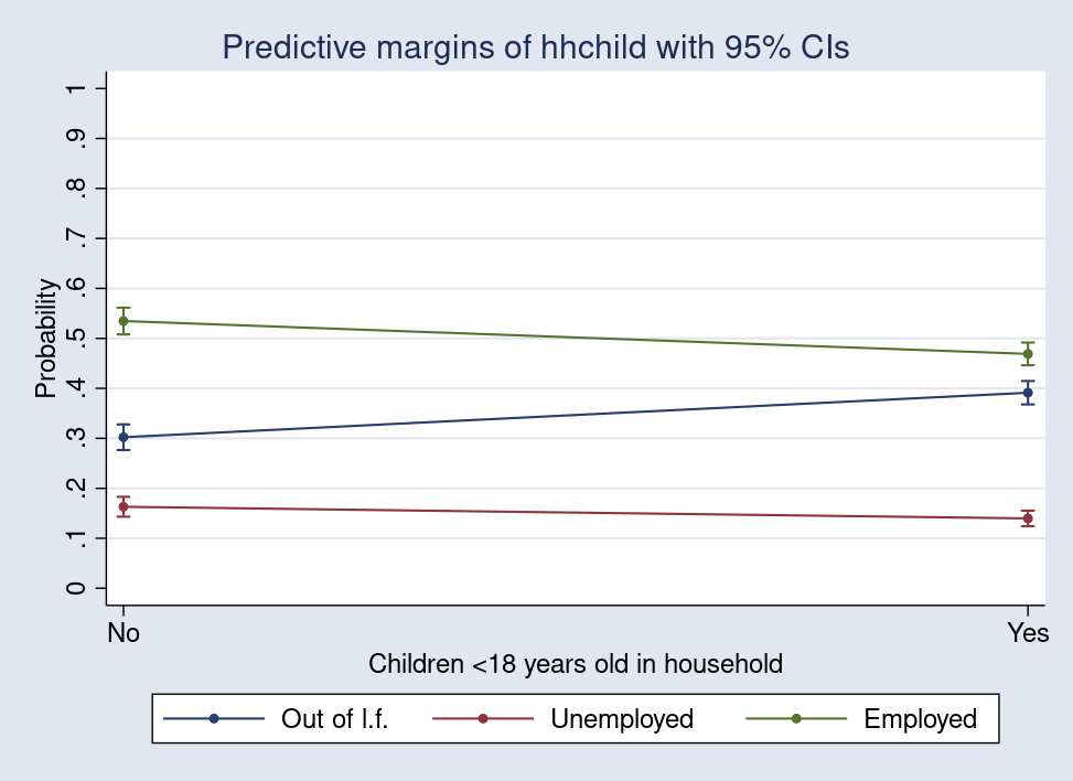
Now we can easily see that the expected probability of being out of the labor force is higher for those with children in the household than for those without. Likewise, the expected probabilities of being unemployed and employed decrease when a child is in the household.
As we have mentioned earlier, if we use the random-effects estimator, we have to be willing to assume that the random effects are uncorrelated with the model covariates. If this assumption does not hold, the random-effects estimator becomes inconsistent. In that case, we may use a conditional fixed-effects estimator, which allows for arbitrary correlation between the unobservable, time-invariant characteristics and the covariates. However, it is worth noting that this added flexibility of the fixed-effects estimator comes at a price. Most notably, because the conditional fixed-effects estimator leaves the individual-level unobservables unestimated, we cannot perform model predictions that account for these unobserved characteristics. In other words, if we use the conditional fixed-effects estimator, we have to rely on the estimated model coefficients or their transforms in the form of the RRR. To fit the conditional fixed-effects multinomial logit model with xtmlogit, we simply add the fe option:
. xtmlogit estatus i.hhchild age hhincome i.hhsigno i.bwinner, fe rrr
note: 80 groups (451 obs) omitted because of no variation in the outcome
      variable over time.

Computing initial values ...

Setting up 26,168 permutations:
....10%....20%....30%....40%....50%....60%....70%....80%....90%....100%

Fitting full model:

Iteration 0:    log likelihood = -2136.5919
Iteration 1:    log likelihood = -2136.2728
Iteration 2:    log likelihood = -2136.2728

Fixed-effects multinomial logistic regression           Number of obs    = 4,310
Group variable: id                                      Number of groups =   720

                                                        Obs per group:
                                                                    min =      5
                                                                    avg =    6.0
                                                                    max =      7

                                                        LR chi2(10)     = 103.29
Log likelihood = -2136.2728                             Prob > chi2     = 0.0000
| estatus | RRR Std. err. z P>|z| [95% conf. interval] | |
| Out_of_lab~e | ||
| hhchild | ||
| Yes | 1.800717 .2266555 4.67 0.000 1.407036 2.304549 | |
| age | .9996159 .0147684 -0.03 0.979 .9710854 1.028985 | |
| hhincome | .9878698 .0087391 -1.38 0.168 .9708891 1.005148 | |
| hhsigno | ||
| Yes | 1.663632 .166548 5.08 0.000 1.367233 2.024287 | |
| bwinner | ||
| Yes | .6277743 .0491447 -5.95 0.000 .5384781 .7318786 | |
| Unemployed | ||
| hhchild | ||
| Yes | 1.177757 .1930267 1.00 0.318 .8541801 1.623911 | |
| age | 1.006356 .0195273 0.33 0.744 .9688014 1.045366 | |
| hhincome | .9706959 .0116513 -2.48 0.013 .9481262 .9938029 | |
| hhsigno | ||
| Yes | 1.124478 .1463356 0.90 0.367 .8713222 1.451187 | |
| bwinner | ||
| Yes | .7795833 .0802992 -2.42 0.016 .637069 .9539784 | |
| Employed | (base outcome) | |
Looking at the output, we can see that there are no random-effects estimates. We can also see that the model does not include constant terms. Inspecting the RRR in the first equation, we find this to be around 1.8. Thus, in this example, the results of the fixed-effects estimator yield a similar conclusion to the random-effects results.
To find out more about xtmlogit, we encourage everyone to have a look at the [XT] xtmlogit documentation, especially the Remarks and examples section. This section also shows how to perform a Hausman test that can aid in the decision of whether to use a random- or fixed-effects estimator.
— by Joerg Luedicke
Senior Social Scientist and Software Developer


