

In the spotlight: Using margins to interpret choice model results
We use discrete choice models to learn about behavioral patterns and decision making. What factors influence people to vote for one candidate over another in an election? Why do people decide to buy a Toyota, Ford, Chevrolet, or Honda? Why do some people live in a big city, while others prefer living in a small village? Below, I want to show you how easy it is to use Stata's commands for discrete choice models in combination with the margins command to explore these types of decision-making behaviors.
Suppose we can choose how we travel to our workplace: do we use a car, a bicycle, or public transportation? Why do some people use a car and others do not? Here is an excerpt of a panel dataset from a (fictitious) transportation study in a metropolitan area where people have the choice between using a car, using public transportation, using a bicycle, and walking, and we observe each person multiple times:
. list id t alt choice trcost trtime age income in 1/12, sepby(t) noobs
| id t alt choice trcost trtime age income | |||
| 1 1 Car 1 4.14 0.13 30.0 30 | |||
| 1 1 Public 0 4.74 0.42 30.0 30 | |||
| 1 1 Bicycle 0 2.76 0.36 30.0 30 | |||
| 1 1 Walk 0 0.92 0.13 30.0 30 | |||
| 1 2 Car 1 8.00 0.14 32.0 50 | |||
| 1 2 Public 0 3.14 0.12 32.0 50 | |||
| 1 2 Bicycle 0 2.56 0.18 32.0 50 | |||
| 1 2 Walk 0 0.64 0.39 32.0 50 | |||
| 1 3 Car 1 1.76 0.18 34.0 50 | |||
| 1 3 Public 0 2.25 0.50 34.0 50 | |||
| 1 3 Bicycle 0 0.92 1.05 34.0 50 | |||
| 1 3 Walk 0 0.58 0.59 34.0 50 | |||
The alternatives are recorded in the variable alt. The binary variable choice records the chosen alternative; choice is 1 for the chosen transportation method and 0 otherwise. For each individual, we have one choice set per time, and the variable t records time. We can see from the data excerpt that this person chose to use the car at all three points in time. Cost of travel (trcost, measured in $ per trip) and travel time (trtime, measured in hours per trip) are alternative-specific variables, which can differ across alternatives, individuals, and time periods. The variables age (in years) and income (annual income measured in $1,000) are case-specific variables, which do not vary across alternatives for a given time and individual.
We would like to get some answers to the following questions:
- How does cost of car travel affect the probability of choosing to commute by car?
- How does cost of car travel affect the probability of choosing any of the other alternatives?
. cmset id t alt
panel data: panels id and time t
note: case identifier _caseid generated from id t
note: panel by alternatives identifier _panelaltid generated from id alt

                     caseid variable:  _caseid
               alternatives variable:  alt
      panel by alternatives variable:  _panelaltid (strongly balanced)
                       time variable:  t, 1 to 3
                               delta:  1 unit

note: data have been xtset
We now use cmxtmixlogit to fit our model. We include travel cost and travel time as covariates with random coefficients. To accommodate a more flexible functional form, we include a squared term for travel cost as well as interaction terms with travel time. We also include case-specific variables age and income as covariates with fixed coefficients.
. cmxtmixlogit choice, random(c.trcost##c.trcost##c.trtime)
               casevars(age income) intpoints(50) nolog


Mixed logit choice model                     Number of obs        =      6,000
                                             Number of cases      =      1,500
Panel variable: id                           Number of panels     =        500

Time variable: t                             Cases per panel: min =          3
                                                              avg =        3.0
                                                              max =          3

Alternatives variable: alt                   Alts per case:   min =          4
                                                              avg =        4.0
                                                              max =          4
Integration sequence:      Hammersley
Integration points:                50             Wald chi2(11)   =     176.30
Log simulated-likelihood = -855.50085             Prob > chi2     =     0.0000
| choice | Coef. Std. Err. z P>|z| [95% Conf. Interval] | |
| alt | ||
| trcost | -2.411053 .309898 -7.78 0.000 -3.018442 -1.803664 | |
| c.trcost# | ||
| c.trcost | .1155629 .0408743 2.83 0.005 .0354507 .195675 | |
| trtime | -2.832468 .6943623 -4.08 0.000 -4.193393 -1.471542 | |
| c.trcost# | ||
| c.trtime | 1.166597 .7131089 1.64 0.102 -.2310708 2.564265 | |
| c.trcost# | ||
| c.trcost# | ||
| c.trtime | -.2371244 .1670896 -1.42 0.156 -.564614 .0903651 | |
| /Normal | ||
| sd(trcost) | 1.128526 .1420839 .8817454 1.444374 | |
| sd(c.trcost# | ||
| c.trcost) | .0738845 .0189857 .0446503 .1222595 | |
| sd(trtime) | 2.348856 .4020465 1.679418 3.285141 | |
| sd(c.trcost# | ||
| c.trtime) | .6655678 .2833858 .2889131 1.533265 | |
| sd(c.trcost# | ||
| c.trcost# | ||
| c.trtime) | .0799671 .0654532 .0160769 .3977604 | |
| Car | (base alternative) | |
| Public | ||
| age | .0167133 .0122569 1.36 0.173 -.0073099 .0407364 | |
| income | -.0808542 .0081533 -9.92 0.000 -.0968344 -.0648741 | |
| _cons | .7772837 .6152141 1.26 0.206 -.4285137 1.983081 | |
| Bicycle | ||
| age | .0308463 .0154651 1.99 0.046 .0005353 .0611574 | |
| income | -.1246103 .0117496 -10.61 0.000 -.147639 -.1015815 | |
| _cons | .2571076 .782674 0.33 0.743 -1.276905 1.79112 | |
| Walk | ||
| age | .0494648 .018721 2.64 0.008 .0127723 .0861572 | |
| income | -.179663 .01517 -11.84 0.000 -.2093957 -.1499304 | |
| _cons | .6208756 .9489958 0.65 0.513 -1.239122 2.480873 | |
But now what? By simply looking at this model output, we cannot get any clear answers to our above questions. Even if we had not included interaction effects or squared terms, the amount of information that can be gathered from just looking at the model coefficients is very limited in a choice model such as the mixed logit. A better way to interpret the results from our model is to go directly after the modeled choice probabilities. To start simply, let's try to answer the following question: if cost of car travel was $4.20 (its average) for every individual, what is the expected proportion of individuals who will select each travel method? To answer this question, we use the following margins specification:
. margins, alternative(Car) at(trcost = 4.2)

Predictive margins                              Number of obs     =      6,000
Model VCE    : OIM

Expression   : Pr(alt), predict()
Alternative  : Car
at           : trcost          =         4.2
| Delta-method | ||
| Margin Std. Err. z P>|z| [95% Conf. Interval] | ||
| _outcome | ||
| Car | .6218004 .0148732 41.81 0.000 .5926495 .6509513 | |
| Public | .1859681 .0099346 18.72 0.000 .1664965 .2054396 | |
| Bicycle | .0969891 .0072537 13.37 0.000 .082772 .1112062 | |
| Walk | .0952424 .0071773 13.27 0.000 .0811752 .1093097 | |
In the above margins specification, we use option alternative(Car) to tell margins that we wish to target the car alternative with respect to the travel cost variable, for which we specify the value of 4.2 in the at() option. We find that, at an average cost of car travel, the expected share of people choosing a car to commute to work is around 0.62, or 62%. The share of people that expect to choose public transportation is around 19%, while using a bicycle or walking to work is least popular with around 10% each.
To get a more complete picture for our questions, however, we would like to see how these proportions are expected to change with cost. To do this, we again compute averaged predicted probabilities for each of the alternatives, but this time we evaluate them over the entire range of car travel cost. We use the following margins specification:
. margins, alternative(Car) at(trcost = (0.5(0.5)8))
<output omitted>
Because we get a lot of output back from margins in this case, it is best to plot the results. We could simply type marginsplot, but we will add a few options for styling and clarity:
. marginsplot, recast(line) ciopts(recast(rarea) color(%20))
               xline(4.2, lpattern(dot) lcolor(gs8) lwidth(0.5))
               xlabel(, format(%2.1f)) ylabel(, angle(0))
               xtitle("Cost of car travel (in $)")
               legend(col(4)) title("")
               text(0.85 5.4 "<-- Average car travel cost",
                    size(*0.8) color(gs6))

  Variables that uniquely identify margins: trcost _outcome
This yields the following graph:
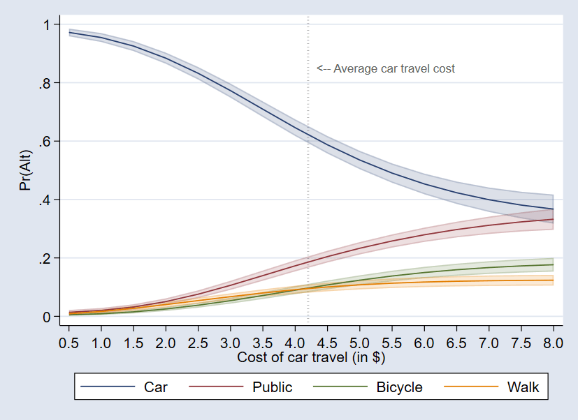
The graph shows the averaged predicted probabilities for each of the alternatives as a function of car travel cost, including 95% confidence bands. Now, we can get a much better idea about how transportation choice is related to car travel cost. As we saw previously, when the cost of car travel is around $4.20, we expect 62% of commuters to take a car, but if this cost is instead $7.00, only around 40% would take the car. We can also see that the chances of choosing any of the other alternatives are increasing with increasing car travel cost, especially for public transportation. For a car travel cost of $8.00, the expected share of car travelers and public transportation commuters is almost the same. On the other end of the spectrum, we can see that, if costs related to using a car were extremely low, almost everybody would use one.
We could do a lot more with margins after choice models, and I encourage everyone to look at Intro 1 of Stata's [CM] Choice Models Reference Manual for a number of introductory examples, as well as the Remarks and examples section of the cmxtmixlogit entry.
— Joerg Luedicke
Senior Social Scientist and Statistician


