

In the spotlight: Interpreting models for log-transformed outcomes
The natural log transformation is often used to model nonnegative, skewed dependent variables such as wages or cholesterol. We simply transform the dependent variable and fit linear regression models like this:
. generate lny = ln(y)
. regress lny x1 x2 ... xk
Unfortunately, the predictions from our model are on a log scale, and most of us have trouble thinking in terms of log wages or log cholesterol. Below, I show you how to use Stata's margins command to interpret results from these models in the original scale. I'm also going to show you an alternative way to fit models with nonnegative, skewed dependent variables.
The data and the model
Let's open the NLSW88 dataset by typing
. sysuse nlsw88.dta
This dataset includes variables for hourly wage (wage), current grade completed (grade), and job tenure measured in years (tenure).
. describe wage grade tenure
| storage display value variable name type format label variable label |
| wage float %9.0g hourly wage grade byte %8.0g current grade completed tenure float %9.0g job tenure (years) |
I would like to fit a linear regression model using grade and tenure as predictors of wage. A summary of the data shows that there are 2,246 observations for hourly wage with a minimum of $1 and a maximum of $40.7.
. summarize wage grade tenure
| Variable | Obs Mean Std. Dev. Min Max | |
| wage | 2,246 7.766949 5.755523 1.004952 40.74659 | |
| grade | 2,244 13.09893 2.521246 0 18 | |
| tenure | 2,231 5.97785 5.510331 0 25.91667 |
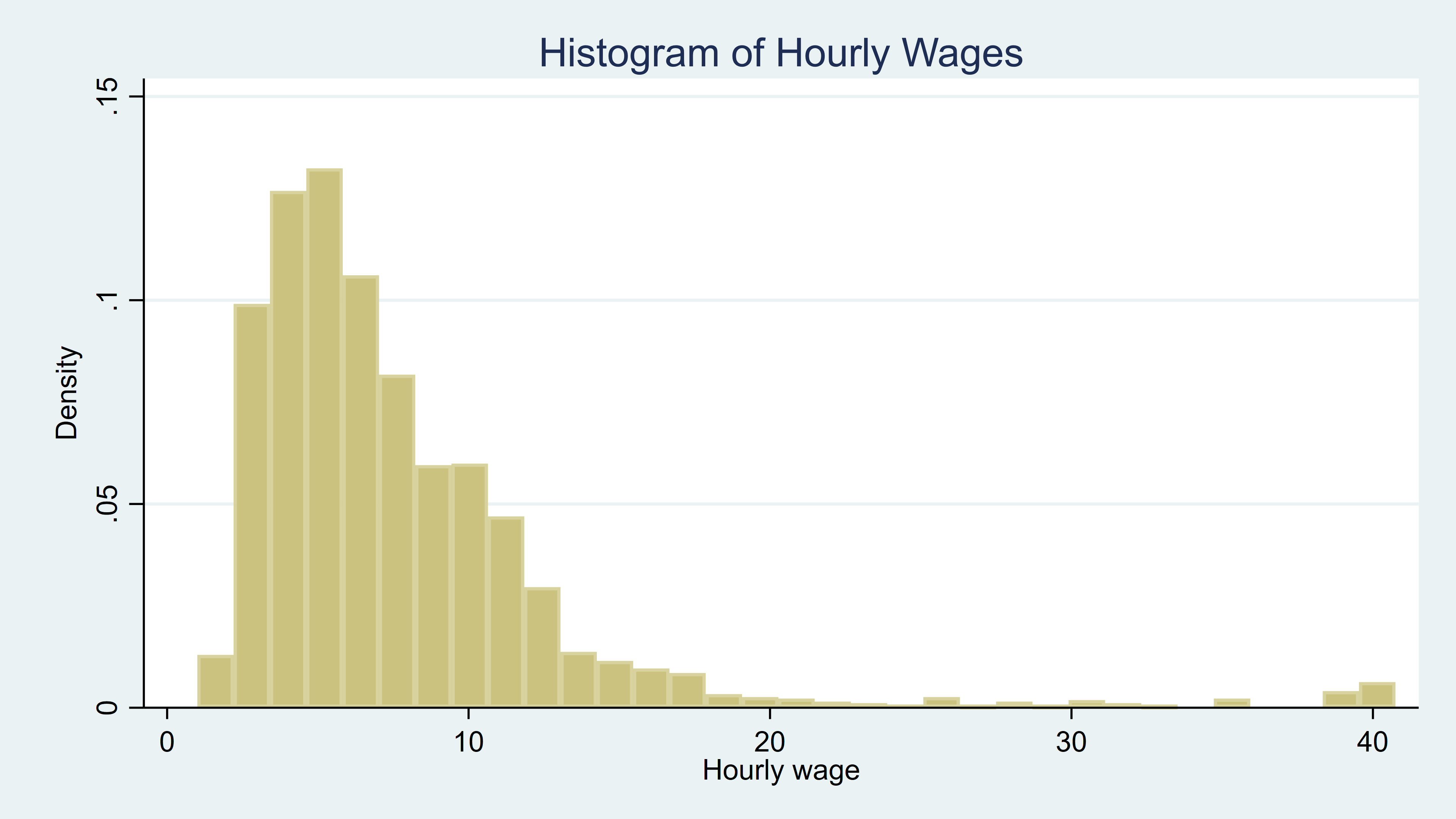
And a histogram shows that wage has a skewed distribution.
. histogram wage, title(Histogram of Hourly Wages)
Let's create a new variable for the natural logarithm of wage.
. generate lnwage = ln(wage)
We can fit a regression model for our transformed variable including grade, tenure, and the square of tenure. Note that I have used Stata's factor-variable notation to include tenure and the square of tenure. The c. prefix tells Stata to treat tenure as a continuous variable, and the ## operator tells Stata to include the main effect (tenure) and the interaction (tenure*tenure).
. regress lnwage grade c.tenure##c.tenure
| Source | SS df MS | Number of obs = 2,229 | |
| F(3, 2225) = 238.31 | |||
| Model | 178.009026 3 59.3363418 | Prob > F = 0.0000 | |
| Residual | 553.998777 2,225 .248988214 | R-squared = 0.2432 | |
| Adj R-squared = 0.2422 | |||
| Total | 732.007802 2,228 .328549283 | Root MSE = .49899 | |
| lnwage | Coef. Std. Err. t P>|t| [95% Conf. Interval] | |
| grade | .0869352 .0042233 20.58 0.000 .0786531 .0952172 | |
| tenure | .0513652 .0062659 8.20 0.000 .0390777 .0636528 | |
| c.tenure#c.tenure | -.0014096 .000336 -4.20 0.000 -.0020685 -.0007508 | |
| _cons | .5201683 .0571766 9.10 0.000 .4080433 .6322934 | |
Now we can use margins to help us interpret the results of our model.
. margins

Predictive margins                              Number of obs     =      2,229
Model VCE    : OLS

Expression   : Linear prediction, predict()
| Delta-method | ||
| Margin Std. Err. t P>|t| [95% Conf. Interval] | ||
| _cons | 1.872838 .010569 177.20 0.000 1.852112 1.893564 | |
This margins command reports the average predicted log wage. Based on this model and assuming we have a random or otherwise representative sample, we expect that the average hourly log wage in the population is 1.87 with a confidence interval of [1.85, 1.89]. However, I'm not sure if that's high or low because I'm not used to thinking on a log-wages scale.
It is tempting to simply exponentiate the predictions to convert them back to wages, but the reverse transformation results in a biased prediction (see references Abrevaya [2002]; Cameron and Trivedi [2010]; Duan [1983]; Wooldridge [2010]).
How to estimate unbiased predictions
Let's assume that the errors from our model are normally distributed and independent of grade and tenure. In this situation, we can remove the bias of the reverse transformation by including a function of the variance of the errors in our prediction,
E(Y|X) = eXBeσ2/2
where σ2 is the variance of the errors.
We can use the square of the root mean squared error (RMSE) as an estimate of the error variance. The RMSE remains in memory after we use regress, and we can refer to it by typing `e(rmse)'. So if we wanted predictions of hourly wages for each individual, we could type
. predict lnwage_hat
. generate wage_hat = exp(lnwage_hat)*exp((`e(rmse)'^2)/2)
Here lnwage_hat is the prediction of log wage, and we plug this into the function above to obtain the predicted wages in wage_hat.
To interpret the results of our model on the wage scale, we will likely want to go beyond these individual-level predictions.
The expression() option in margins
Fortunately, we can use margins with the expresssion() option to compute margins and estimate effects based on a transformation of predictions. In the expression() option, we can refer to the linear prediction of log wage as predict(xb). Our first instinct might be to use the same expression we used in our generate command above and estimate the expected average hourly wage by typing
. margins, expression(exp(predict(xb))*exp((`e(rmse)'^2)/2))
However, the standard error of our estimate will be incorrect. Because regress reports the RMSE but does not estimate its variance, the result of this margins command would include the RMSE as though it were a known value, measured without error. Fortunately, there is a way around this.
How to obtain unbiased estimates and their standard errors
Let's fit our linear regression model using Stata's gsem command.
. gsem lnwage <- grade c.tenure##c.tenure

Iteration 0:   log likelihood = -1611.2674
Iteration 1:   log likelihood = -1611.2674

Generalized structural equation model           Number of obs     =      2,229
Response       : lnwage
Family         : Gaussian
Link           : identity
Log likelihood = -1611.2674
| Coef. Std. Err. z P>|z| [95% Conf. Interval] | ||
| lnwage | ||
| grade | .0869352 .0042195 20.60 0.000 .0786651 .0952053 | |
| tenure | .0513652 .0062602 8.20 0.000 .0390954 .0636351 | |
| c.tenure#c.tenure | -.0014096 .0003357 -4.20 0.000 -.0020675 -.0007517 | |
| _cons | .5201683 .0571253 9.11 0.000 .4082048 .6321318 | |
| var(e.lnwage) | .2485414 .0074449 .2343697 .26357 | |
Notice that the variance of the errors (var(e.lnwage)) is included at the bottom of the output. gsem also estimated the standard error of that variance, and margins will incorporate that standard error into its calculations. In the margins command below, I have replaced xb with eta and `e(rmse)'^2 with _b[/var(e.lnwage)].
. margins, expression(exp(predict(eta))*(exp((_b[/var(e.lnwage)])/2)))

Predictive margins                              Number of obs     =      2,229
Model VCE    : OIM

Expression   : exp(predict(eta))*(exp((_b[/var(e.lnwage)])/2))
| Delta-method | ||
| Margin Std. Err. z P>|z| [95% Conf. Interval] | ||
| _cons | 7.670231 .0889464 86.23 0.000 7.4959 7.844563 | |
Now the results are easier to interpret—the expected average wage is $7.67 per hour. Our standard error and confidence interval are also on the original wage scale.
With these predictions correctly incorporated in the expression() option, we can answer many additional interesting questions using margins. For instance, we can use the at() option to estimate expected hourly wages for different values of the independent variables. For example, what is the expected hourly wage if we set grade at values ranging from 12 to 18 years of education?
. margins, expression(exp(predict(eta))*(exp((_b[/var(e.lnwage)])/2)))
         at(grade=(12(1)18))
  (output omitted)

. marginsplot, title(Expected hourly wage) ytitle(Expected hourly wage) xtitle(Grade completed)
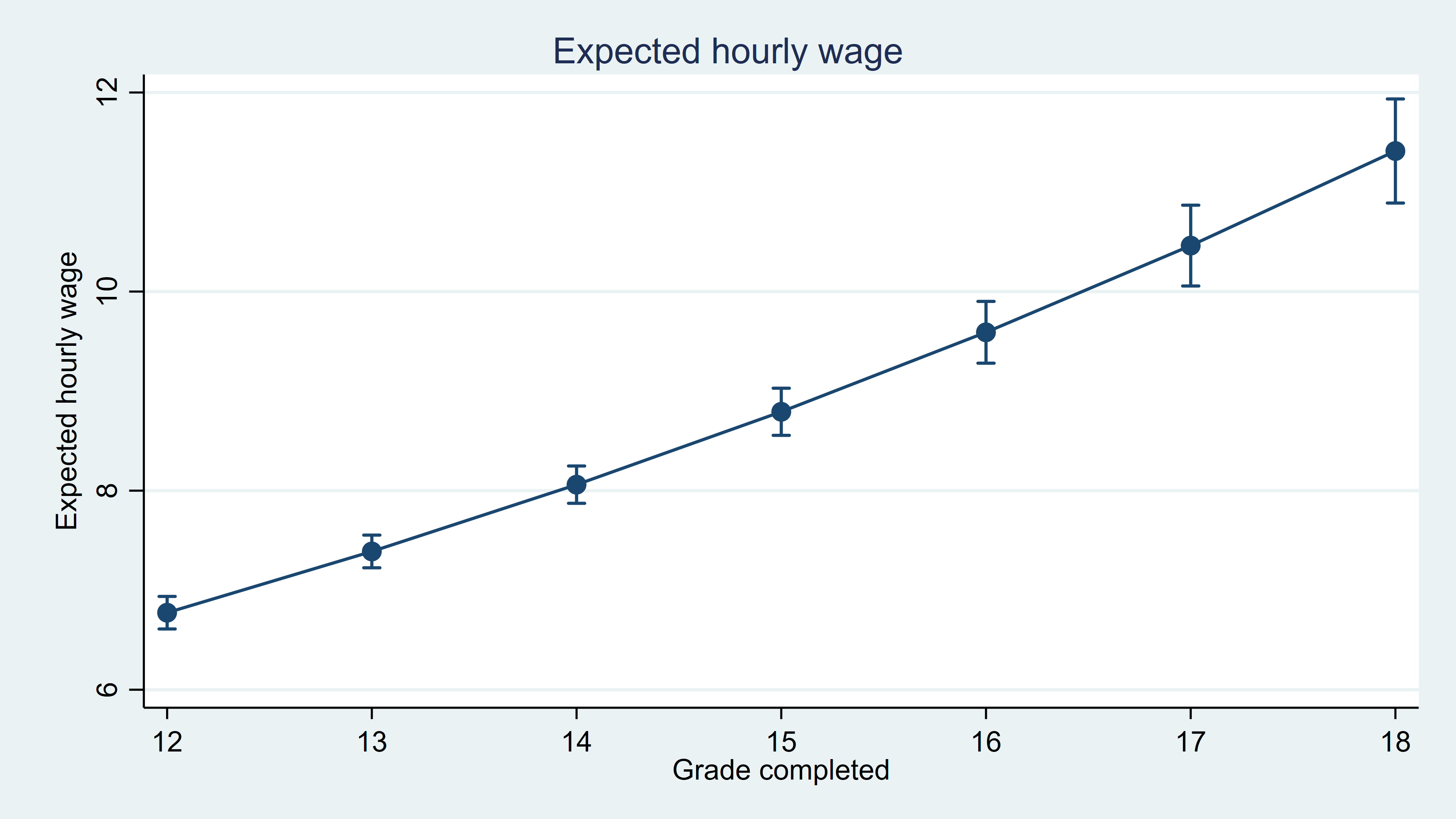
Taking the difference between these values, say, the difference between the expected value when grade=16 and when grade=12, gives us the effect of having a college education instead of a high school education on hourly wages.
Use poisson rather than regress; tell a friend
Bill Gould wrote a blog post in 2011 titled "Use poisson rather than regress; tell a friend". He recommends that we abandon the practice of linear regression with log-transformed dependent variables and instead use Poisson regression with robust standard errors. I won't reiterate his reasoning here, but I will show you how to use this method.
First, we use poisson with the option vce(robust) to fit the model for the untransformed dependent variable wage.
. poisson wage grade c.tenure##c.tenure, vce(robust)
note: you are responsible for interpretation of noncount dep. variable

Iteration 0:   log pseudolikelihood = -7031.0432
Iteration 1:   log pseudolikelihood = -7031.0432

Poisson regression                              Number of obs     =      2,229
                                                Wald chi2(3)      =     402.22
                                                Prob > chi2       =     0.0000
Log pseudolikelihood = -7031.0432               Pseudo R2         =     0.0785
| Robust | ||
| wage | Coef. Std. Err. z P>|z| [95% Conf. Interval] | |
| grade | .0892778 .0053181 16.79 0.000 .0788546 .0997011 | |
| tenure | .0355083 .0082201 4.32 0.000 .0193972 .0516193 | |
| c.tenure#c.tenure | -.0009674 .0004192 -2.31 0.021 -.001789 -.0001458 | |
| _cons | .7013102 .0760402 9.22 0.000 .5522742 .8503462 | |
Then, we use margins just as we did above to estimate the average hourly wage.
. margins

Predictive margins                              Number of obs     =      2,229
Model VCE    : Robust

Expression   : Predicted number of events, predict()
| Delta-method | ||
| Margin Std. Err. z P>|z| [95% Conf. Interval] | ||
| _cons | 7.794419 .1142376 68.23 0.000 7.570517 8.01832 | |
We can again use margins, at() to obtain estimates for different values of grade.
. margins, at(grade=(12(1)18))
  (output omitted)

. marginsplot, title(Expected hourly wage) ytitle(Expected hourly wage) xtitle(Grade completed)

With regress, we made the assumption that the errors were normal. If that assumption is valid, the estimates we obtain using that method are more efficient. However, this approach that uses poisson is more robust.
Whether you use a log transform and linear regression or you use Poisson regression, Stata's margins command makes it easy to interpret the results of a model for nonnegative, skewed dependent variables.
— Chuck Huber
Associate Director of Statistical Outreach
References
- Abrevaya, J. 2002. Computing marginal effects in the Box–Cox model. Econometric Reviews 21: 383–393.
- Cameron, A. C., and P. K. Trivedi. 2010. Microeconometrics Using Stata. Rev. ed. College Station, TX: Stata Press.
- Duan, N. 1983. Smearing estimate: A nonparametric retransformation method. Journal of the American Statistical Association 78: 605-610.
- Wooldridge. J. M. 2010. Econometric Analysis of Cross Section and Panel Data. 2nd ed. Cambridge, MA: MIT Press.


