

Create Word documents: Starring putdocx
Suppose you have just fit several regression models. You want to create a table that presents different specifications and uses asterisks to "star" significant coefficients. Wouldn't it be nice if Stata had a command that let you do this easily?
It does. It has had one for a while. It is called estimates table.
Now suppose you are writing a Word document and you want to put that same table of regression results in it. Ah, well, until now, you couldn't.
The new putdocx command lets you do just that though. Better still, you do not have to learn a lot of complicated programming to do it.
A quick illustration
In this toy example, let's use the auto dataset—that perennial favorite of the Stata manuals.
. webuse auto
We'll start by fitting two regression models. The first model specifies price only as a function of the mileage (mpg) of the car. The second adds an indicator for whether the car was imported from outside the U.S. (foreign). We don't care much about the default regress output, so we'll fit these models quietly.
. quietly regress price mpg
. estimates store model1

. quietly regress price mpg i.foreign
. estimates store model2
Notice that after we fit each model above, we stored the estimation results. We did this so that we could tell estimates table what to display.
. estimates table model1 model2
| Variable | model1 model2 | |
| mpg | -238.89435 -294.19553 | |
| foreign | ||
| Foreign | 1767.2922 | |
| _cons | 11253.061 11905.415 | |
So that's our basic estimates table. Let's customize it to show the contents we want with the format we want. We can format the point estimates of the coefficients to have three decimal places by specifying the b() option. And we can add significance stars at the 95, 99, and 99.9 percent confidence levels with the star option.
. estimates table model1 model2, b(%10.3f) star
| Variable | model1 model2 | |
| mpg | -238.894*** -294.196*** | |
| foreign | ||
| Foreign | 1767.292* | |
| _cons | 11253.061*** 11905.415*** | |
We could stop right here and write our results out. But this probably isn't a table that is good enough for publication just yet. Let's add a few statistics and put in the variable labels rather than names.
. estimates table model1 model2, b(%10.3f) star stats(N r2 r2_a)
    varlabel allbaselevels
| Variable | model1 model2 | |
| Mileage (mpg) | -238.894*** -294.196*** | |
| Car type | ||
| Domestic | (base) | |
| Foreign | 1767.292* | |
| Constant | 11253.061*** 11905.415*** | |
| N | 74 74 | |
| r2 | 0.220 0.284 | |
| r2_a | 0.209 0.264 | |
We feel pretty good about this table. All the content we want to display is there.
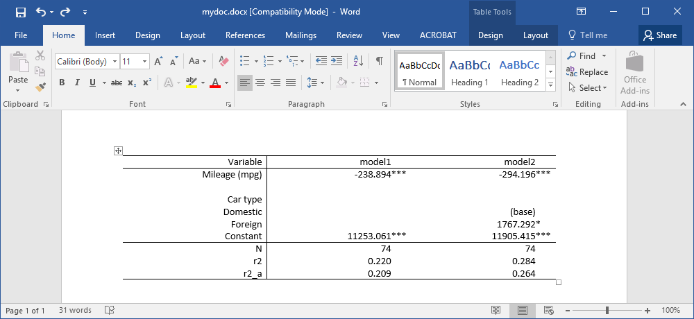
So let's write this to our Word document. We need only three steps: create a document in memory, write out our table, and save the document. We have to specify a table name (tbl1) and a name for our document (mydoc).
. putdocx begin
. putdocx table tbl1 = etable
. putdocx save mydoc
These three commands re-create the table of estimates in Word. Note that if mydoc.docx had existed already, we would have had to specify either the replace or the append option.
Customizing the table in Word
If we are creating a table for one-time use in a publication and not worried about replicating results later, we might hand-edit the results in Word to get a fully polished, publication-ready table. But if we want a reproducible table or if we plan to run similar models again with different data, we are better served by editing our table in Stata and saving the commands in a do-file.
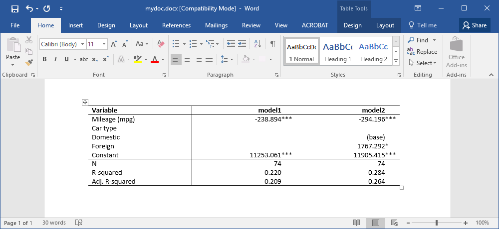
Our goal is to create a table that looks like this:
To do this, we start from the same place above: open a document in memory, and write our estimates table results to a table.
. putdocx begin
. putdocx table tbl2 = etable
tbl2 is just the name we will use to refer to the results while we work with them.
Now we can start modifying our table.
We delete the blank line between "Mileage (mpg)" and "Car type" by removing the third row of the table.
. putdocx table tbl2(3,.), drop
We format the leftmost column to be left aligned and format the header row to be bold.
. putdocx table tbl2(.,1), halign(left)
. putdocx table tbl2(1,.), bold
Finally, we give labels to the r2 and r2_a statistics and then add the formatted table to our existing document.
. putdocx table tbl2(8,1) = ("R-squared")
. putdocx table tbl2(9,1) = ("Adj. R-squared")
. putdocx save mydoc, append
If we want to devote some extra time to programming, we could create even more complicated tables. See [RPT] putdocx and [RPT] putpdf for other ways to create tables with these commands.
While we have concentrated on tables of regression results, you can also use putdocx (for Word documents) and putpdf (for PDF files) to automate the production of entire reports. Directly from within Stata, you can create documents containing paragraphs, tables, embedded Stata output, and Stata graphs and other graphics, with full control over formatting such as font size, typeface, and the like.
— Rebecca Raciborski
Senior Health Econometrician


