
Markov-switching models
- Markov transition modeling
- Autoregressive model
- Dynamic regression model
- State-dependent variance parameters
- Tables of
- Transition probabilities
- Expected state durations
- Predictions
- Expected values of dependent variable
- Probabilities of being in a state
- Static (one-step)
- Dynamic (multistep)
- RMSEs of predictions
Markov switching is about time-series models in which the parameters change over time between regimes, and the switching is either abrupt or smooth. Smooth switching is achieved by autoregressively smoothing the transition. Abrupt switching is called dynamic. When the switching occurs is unknown, as are the number of switching points. The number of regimes is known.
Markov-switching models have been used to study asymmetric behavior of recessions and expansions; recessions happen fast, subsequent expansions, more slowly. They have been used for many other problems as well.
Say we have data on the incidence of mumps per 10,000 residents in New York City between 1928 and 1972.
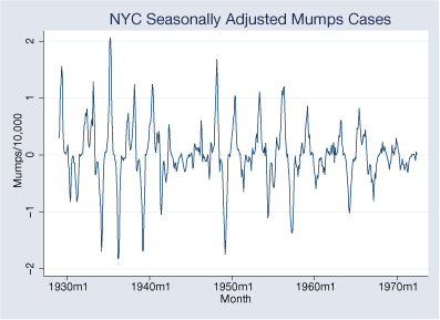
There are periods of high and low volatility. The volatility is sometimes greater than at other times, and we are going to look at that. We are going to assume two regimes and fit a dynamic (abrupt-change) model.
. mswitch dr S12.mumpspc,
  varswitch switch(LS12.mumpspc, noconstant)
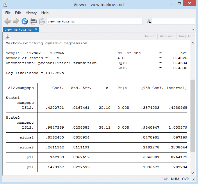
Note the two variance parameters sigma1 and sigma2. They confirm our intuition of low- and high-variance regimes.
Note the two transition probability terms p11 and p21. This is the Markov transition model. The full set of transition probabilities is as follows:
| from/to state | 1 | 2 |
| 1 | 0.76 | 1−0.76 |
| 2 | 0.15 | 1−0.15 |
The states are persistent. State 1 transits to state 1 with probability 0.76. State 2 transits to state 2 with probability 0.85 (1 − 0.15).


