Learn about structural equation modeling (SEM).
Model specification
- Use the SEM Builder or command language

- SEM Builder uses standard path diagrams
- Command language is a natural variation on path diagrams
- Group estimation is as easy as adding group(sex). Also easily
add or relax constraints—ginvariant(mcoef) constrains
all coefficients in the measurement model to be equal across groups.
Or add paths for some groups but not others.
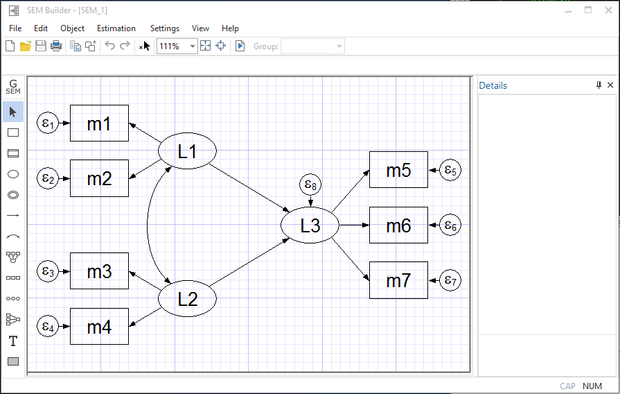
SEM Builder
- Drag, drop, and connect to create path diagrams
- Estimate models from path diagrams
- Display results on the path diagram
- Save and modify diagrams
- Tools to create measurement and regression components
- Set constant and equality constraints by clicking
- Complete control of how your diagrams look
Classes of models for linear SEM
- Linear regression
- Multivariate regression
- Path analysis
- Mediation analysis
- Measurement models
- Confirmatory factor analysis (CFA)
- Multiple indicators and multiple causes (MIMIC) models
- Latent growth curve models
- Hierarchical CFA
- Correlated uniqueness models
- Arbitrary structural equation models
Additional classes of models for generalized SEM
- Generalized linear models
- Item response theory models
- Measurement models with binary, count, and ordinal measurements
- Multilevel CFA models
- Multilevel mixed-effects models
- Latent growth curve models with generalized-linear responses
- Multilevel mediation models
- Latent class analysis (LCA) Updated
- Selection models
- with random intercepts and slopes
- with binary, count, and ordinal outcomes
- Endogenous treatment-effect models
- Any multilevel structural equation models with
generalized-linear responses
Structural equation models with survival outcomes
- Latent predictors of survival outcomes
- Path models, growth curve models, and more
- Weibull, exponential, lognormal, loglogistic, or gamma models
- Survival outcomes with other outcomes
Linear and generalized-linear responses
- Models for continuous, binary, count, ordinal, and nominal outcomes
- Thirteen distribution families
- Gaussian
- Bernoulli
- Binomial
- Poisson
- Negative binomial
- Ordinal
- Multinomial
- Beta
- Exponential
- Gamma
- Lognormal
- Loglogistic
- Weibull
- Five links
- Identity
- Log
- Logit
- Probit
- Cloglog
- Support for common regression models: linear, logistic, probit, ordered
logit, ordered probit, Poisson, multinomial logistic, tobit, interval measurements, and more
Multilevel models
- Two-, three-, and higher-level structural equation models
- Multilevel mixed-effects models
- Random intercepts and random slopes
- Crossed and nested random effects
Estimation methods for linear SEM
- ML—maximum likelihood
- MLMV—maximum likelihood for missing values; sometimes called FIML
- ADF—asymptotic distribution free, meaning GMM (generalized method of
moments) using ADF weighting matrix
Estimation methods for generalized SEM
- Maximum likelihood
- Mean-variance or mode-curvature adaptive Gauss–Hermite quadrature
- Nonadaptive Gauss–Hermite quadrature
- Laplace approximation
Standard-error methods
- OIM—observed information matrix
- EIM—expected information matrix
- OPG—outer product of gradients
- Satorra—Bentler estimator
- Robust—distribution-free linearized estimator
- Cluster–robust—robust adjusting for correlation within groups of
observations
- Bootstrap—nonparametric bootstrap and clustered bootstrap
- Jackknife—delete-one, delete-n, and clustered jackknife
Survey support for linear SEM and generalized SEM
- Sampling weights and stage-level weights
- Stratification and poststratification
- Clustered sampling at one or more levels
Postestimation Selector
- View and run all postestimation features for your command
- Automatically updated as estimation commands are run
Summary statistics data (SSD)
- Fit linear SEMs on observed or summary (SSD) data
- Fit models on covariances or correlations and optionally variances and
means
- SSD may be group specific
- Easily create and manage SSDs
- Build SSDs from original (raw) data for distribution or publication
- Automatic corruption/error checking and repairing
- Electronic signatures
Starting values
- Automatic
- May specify for some or all parameters
- Grid search available
- May fit one model, subset or superset, and use fitted values for another model
Identification
- Automatic normalization (anchoring) constraints provide scale for latent
variables; may be overridden
Reliability
- May specify fraction of variance not due to measurement error
Direct and indirect effects for linear SEM
- Confidence intervals
- Unstandardized or standardized units
Overall goodness-of-fit statistics for linear SEM
- Model vs. saturated
- Baseline vs. saturated
- RMSEA, root mean squared error of approximation
- AIC, Akaike's information criterion
- BIC, Bayesian information criterion
- CFI, comparative fit index
- TLI, Tucker–Lewis index, a.k.a. nonnormed fit index
- SRMR, standardized root mean squared residual
- CD, coefficient of determination
Equation-level goodness-of-fit statistics for linear SEM
- R-squared
- Equation-level variance decomposition
- Bentler–Raykov squared multiple-correlation coefficient
Group-level goodness-of-fit statistics for linear SEM
- SRMR
- CD
- Model vs. saturated chi-squared contribution
Residual analysis for linear SEM
- Mean residuals
- Variance and covariance residuals
- Raw, normalized, and standardized values available
Parameter tests
- Modification indices
- Wald tests
- Score tests
- Likelihood-ratio tests
- Easy to specify single or joint custom tests for omitted paths, included
paths, and relaxing constraints
- Linear and nonlinear tests of estimated parameters
- Tests may be specified in standardized or unstandardized parameter units
Group-level parameter tests
- Group invariance by parameter class or user specified
Linear and nonlinear combinations of estimated parameters
- Confidence intervals
- Unstandardized or standardized units
Assess nonrecursive system stability
Predictions for linear SEM
- Observed endogenous variables
- Latent endogenous variables
- Latent variables (factor scores)
- Equation-level first derivatives
- In- and out-of-sample prediction; may estimate on one sample and form
predictions in another
Predictions for generalized SEM
- Means of observed endogenous variables—probabilities for 0/1
outcomes, mean counts, etc.
- Linear predictions of observed endogenous variables
- Latent variables using empirical Bayes means and modes
- Standard errors of empirical Bayes means and modes
- Observed endogenous variables with and without
predictions of latent variables
- Density function
- Distribution function
- Survivor function
- Predict observed endogenous variables marginally with respect to latent variables
- User-defined nonlinear predictions
Results
- May be used with postestimation features
- May be saved to disk for restoration and use later
- Displayed in standardized or unstandardized units
- Optionally display results in Bentler–Weeks form
- Optionally display results in exponentiated form as odds ratios,
incidence rate ratios, and relative risk ratios
- All results accessible for community-contributed programs
Factor variables with generalized SEM
- Automatically create indicators based on categorical variables
- Form interactions among discrete and continuous variables
- Include polynomial terms
- Perform contrasts of categories/levels
Marginal analysis
Contrasts for generalized SEM
- Analysis of main effects, simple effects, interaction effects, partial
interaction effects, and nested effects
- Comparisons against reference groups, of adjacent levels, or against the
grand mean
- Orthogonal polynomials
- Helmert contrasts
- Custom contrasts
- ANOVA-style tests
- Contrasts of nonlinear responses
- Multiple-comparison adjustments
- Balanced and unbalanced data
- Contrasts of means, intercepts, and slopes
- Graphs of contrasts
- Interaction plots
Pairwise comparisons for generalized SEM
- Compare estimated means, intercepts, and slopes
- Compare marginal means, intercepts, and slopes
- Balanced and unbalanced data
- Nonlinear responses
- Multiple-comparison adjustments: Bonferroni, Sidak, Scheffe, Tukey HSD,
Duncan, and Student–Newman–Keuls adjustments
- Group comparisons that are significant
- Graphs of pairwise comparisons
Explore more about SEM in Stata.
Additional resources

)


